Case Study 2 EDA

Import Data

data = read.csv('/Users/elyjiahpotter/Desktop/DDS-Project-2/CaseStudy2-data.csv')

head(data)

##   ID Age Attrition    BusinessTravel DailyRate             Department DistanceFromHome Education   EducationField EmployeeCount
## 1  1  32        No     Travel_Rarely       117                  Sales               13         4    Life Sciences             1
## 2  2  40        No     Travel_Rarely      1308 Research & Development               14         3          Medical             1
## 3  3  35        No Travel_Frequently       200 Research & Development               18         2    Life Sciences             1
## 4  4  32        No     Travel_Rarely       801                  Sales                1         4        Marketing             1
## 5  5  24        No Travel_Frequently       567 Research & Development                2         1 Technical Degree             1
## 6  6  27        No Travel_Frequently       294 Research & Development               10         2    Life Sciences             1
##   EmployeeNumber EnvironmentSatisfaction Gender HourlyRate JobInvolvement JobLevel                JobRole JobSatisfaction MaritalStatus
## 1            859                       2   Male         73              3        2        Sales Executive               4      Divorced
## 2           1128                       3   Male         44              2        5      Research Director               3        Single
## 3           1412                       3   Male         60              3        3 Manufacturing Director               4        Single
## 4           2016                       3 Female         48              3        3        Sales Executive               4       Married
## 5           1646                       1 Female         32              3        1     Research Scientist               4        Single
## 6            733                       4   Male         32              3        3 Manufacturing Director               1      Divorced
##   MonthlyIncome MonthlyRate NumCompaniesWorked Over18 OverTime PercentSalaryHike PerformanceRating RelationshipSatisfaction StandardHours
## 1          4403        9250                  2      Y       No                11                 3                        3            80
## 2         19626       17544                  1      Y       No                14                 3                        1            80
## 3          9362       19944                  2      Y       No                11                 3                        3            80
## 4         10422       24032                  1      Y       No                19                 3                        3            80
## 5          3760       17218                  1      Y      Yes                13                 3                        3            80
## 6          8793        4809                  1      Y       No                21                 4                        3            80
##   StockOptionLevel TotalWorkingYears TrainingTimesLastYear WorkLifeBalance YearsAtCompany YearsInCurrentRole YearsSinceLastPromotion
## 1                1                 8                     3               2              5                  2                       0
## 2                0                21                     2               4             20                  7                       4
## 3                0                10                     2               3              2                  2                       2
## 4                2                14                     3               3             14                 10                       5
## 5                0                 6                     2               3              6                  3                       1
## 6                2                 9                     4               2              9                  7                       1
##   YearsWithCurrManager
## 1                    3
## 2                    9
## 3                    2
## 4                    7
## 5                    3
## 6                    7

Check for missing values

gg_miss_var(data)

## Warning: It is deprecated to specify `guide = FALSE` to remove a guide. Please use `guide = "none"` instead.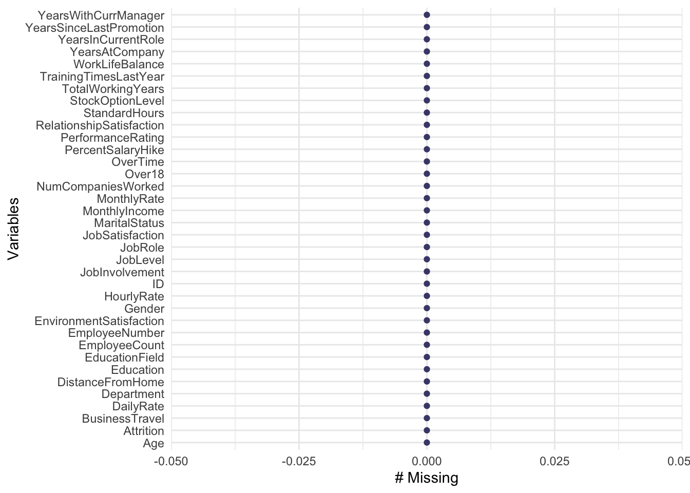

Adjust Attrition Variable for Modeling

data =data %>%
  mutate(Attr = case_when( Attrition == "Yes" ~ 1,
                           Attrition == "No" ~ 0))

Investigate Distributions of Potentially Relevant Discrete Variablees

data %>% ggplot(aes(x = Age, fill = Attrition)) + geom_boxplot()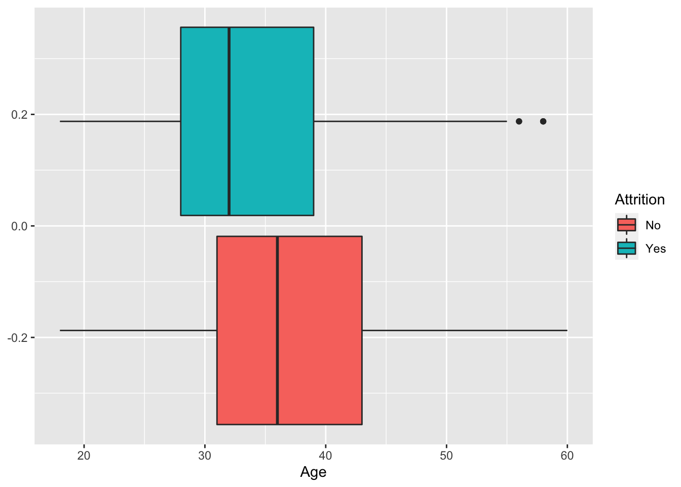

data %>% ggplot(aes(x = DailyRate, fill = Attrition)) + geom_boxplot()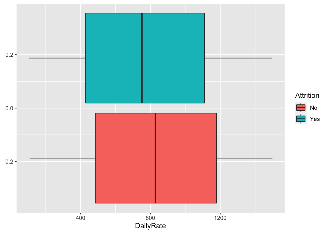

data %>% ggplot(aes(x = DistanceFromHome, fill = Attrition)) + geom_boxplot()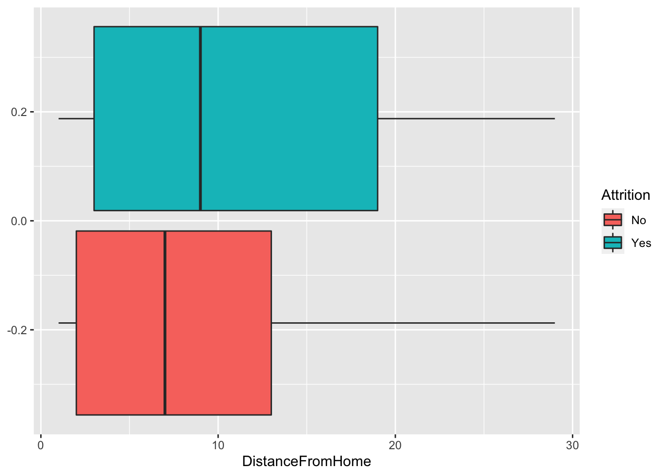

data %>% ggplot(aes(x = Education, fill = Attrition)) + geom_boxplot()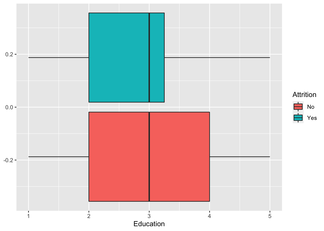

data %>% ggplot(aes(x = EnvironmentSatisfaction, fill = Attrition)) + geom_boxplot()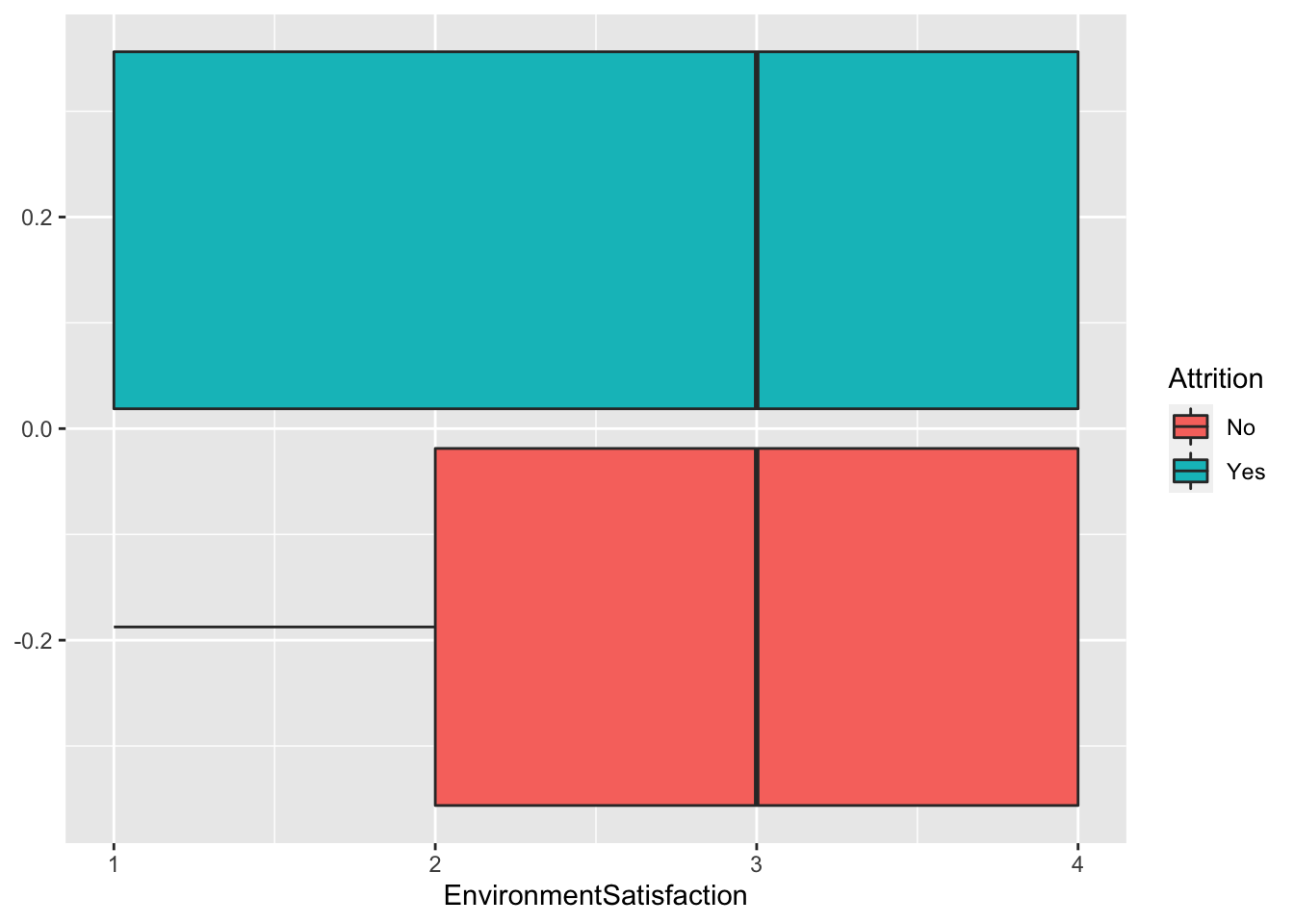

data %>% ggplot(aes(x = HourlyRate, fill = Attrition)) + geom_boxplot()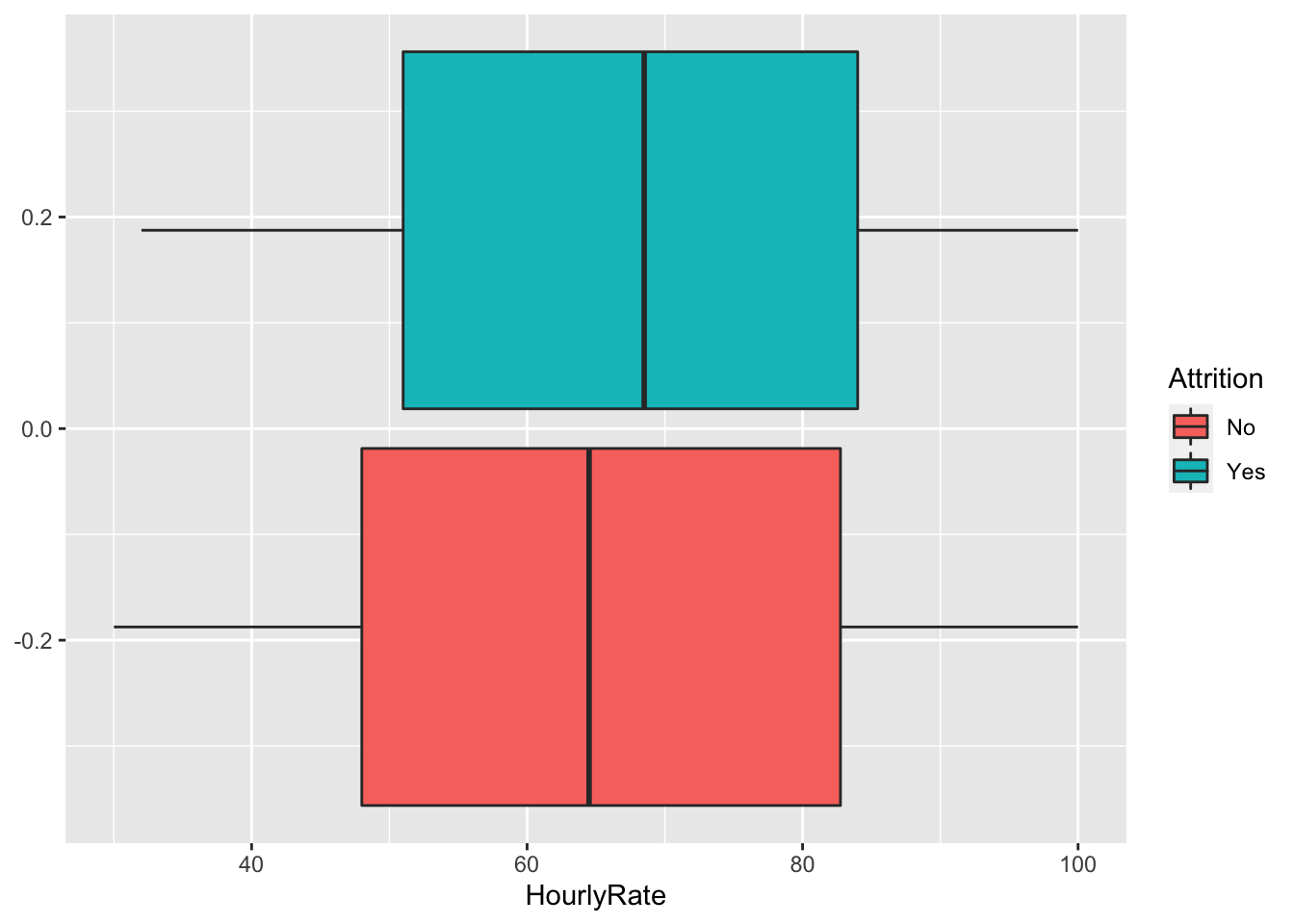

data %>% ggplot(aes(x = JobInvolvement, fill = Attrition)) + geom_boxplot()

data %>% ggplot(aes(x = JobLevel, fill = Attrition)) + geom_boxplot()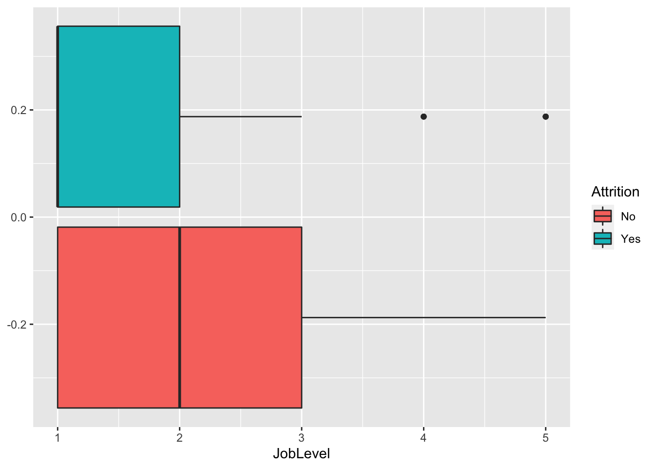

data %>% ggplot(aes(x = JobSatisfaction, fill = Attrition)) + geom_boxplot()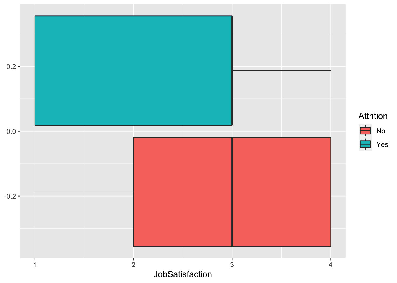

data %>% ggplot(aes(x = MonthlyIncome, fill = Attrition)) + geom_boxplot()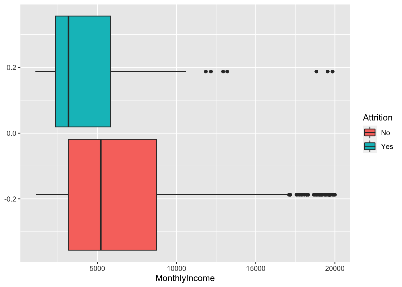

data %>% ggplot(aes(x = MonthlyRate, fill = Attrition)) + geom_boxplot()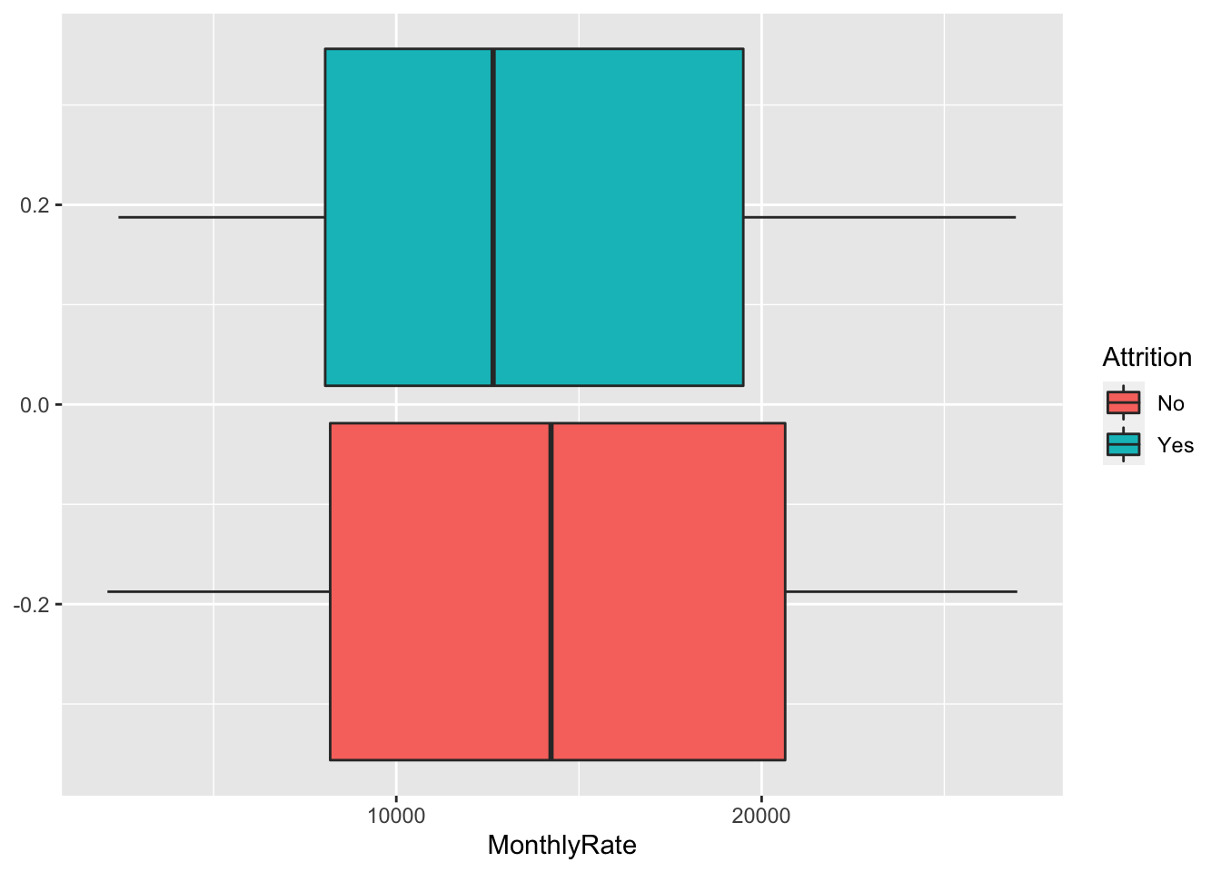

data %>% ggplot(aes(x = NumCompaniesWorked, fill = Attrition)) + geom_boxplot()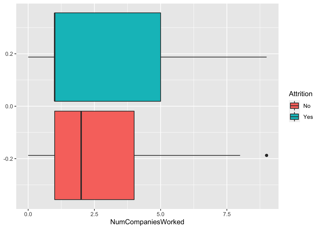

data %>% ggplot(aes(x = PercentSalaryHike, fill = Attrition)) + geom_boxplot()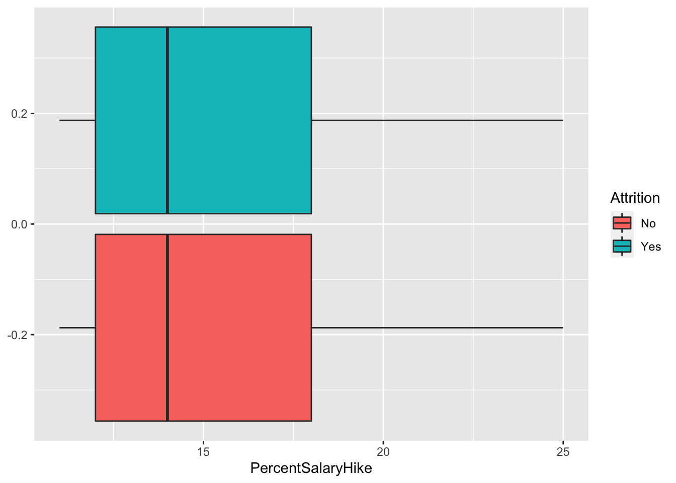

data %>% ggplot(aes(x = RelationshipSatisfaction, fill = Attrition)) + geom_boxplot()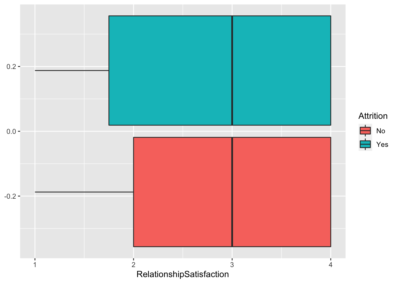

data %>% ggplot(aes(x = StockOptionLevel, fill = Attrition)) + geom_boxplot()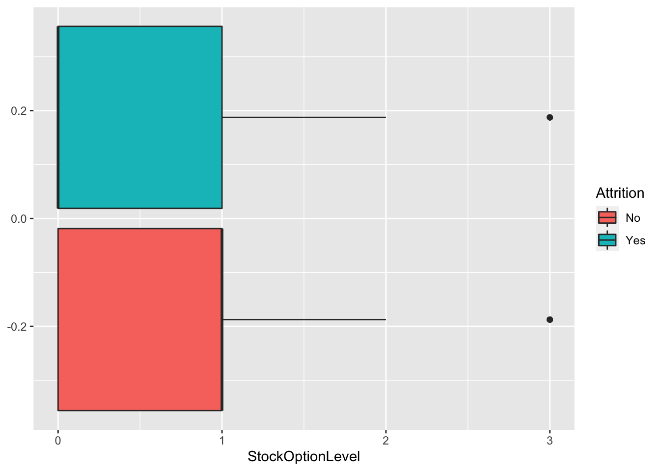

data %>% ggplot(aes(x = TotalWorkingYears, fill = Attrition)) + geom_boxplot()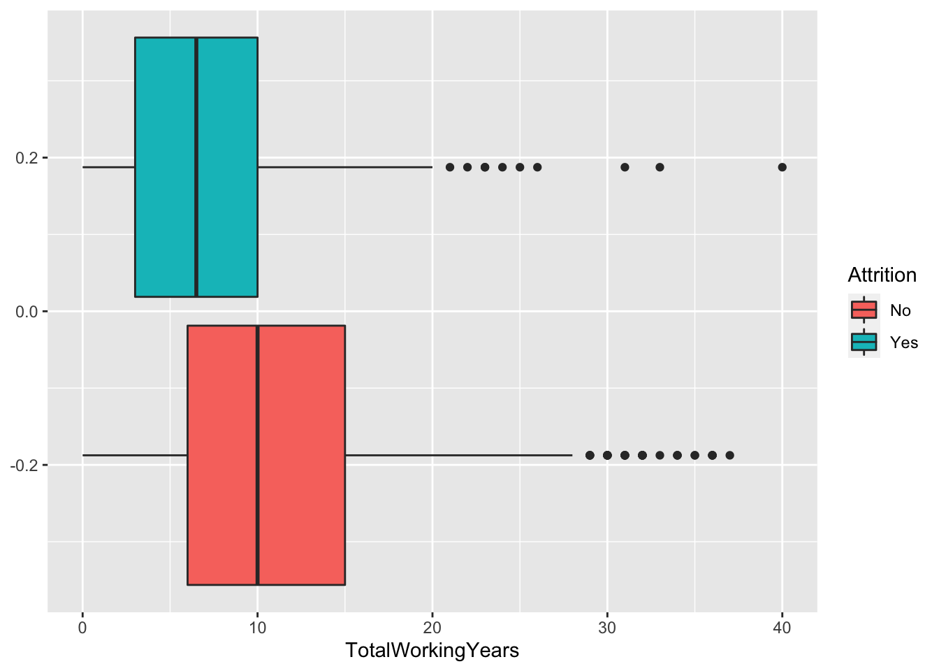

data %>% ggplot(aes(x = TrainingTimesLastYear, fill = Attrition)) + geom_boxplot()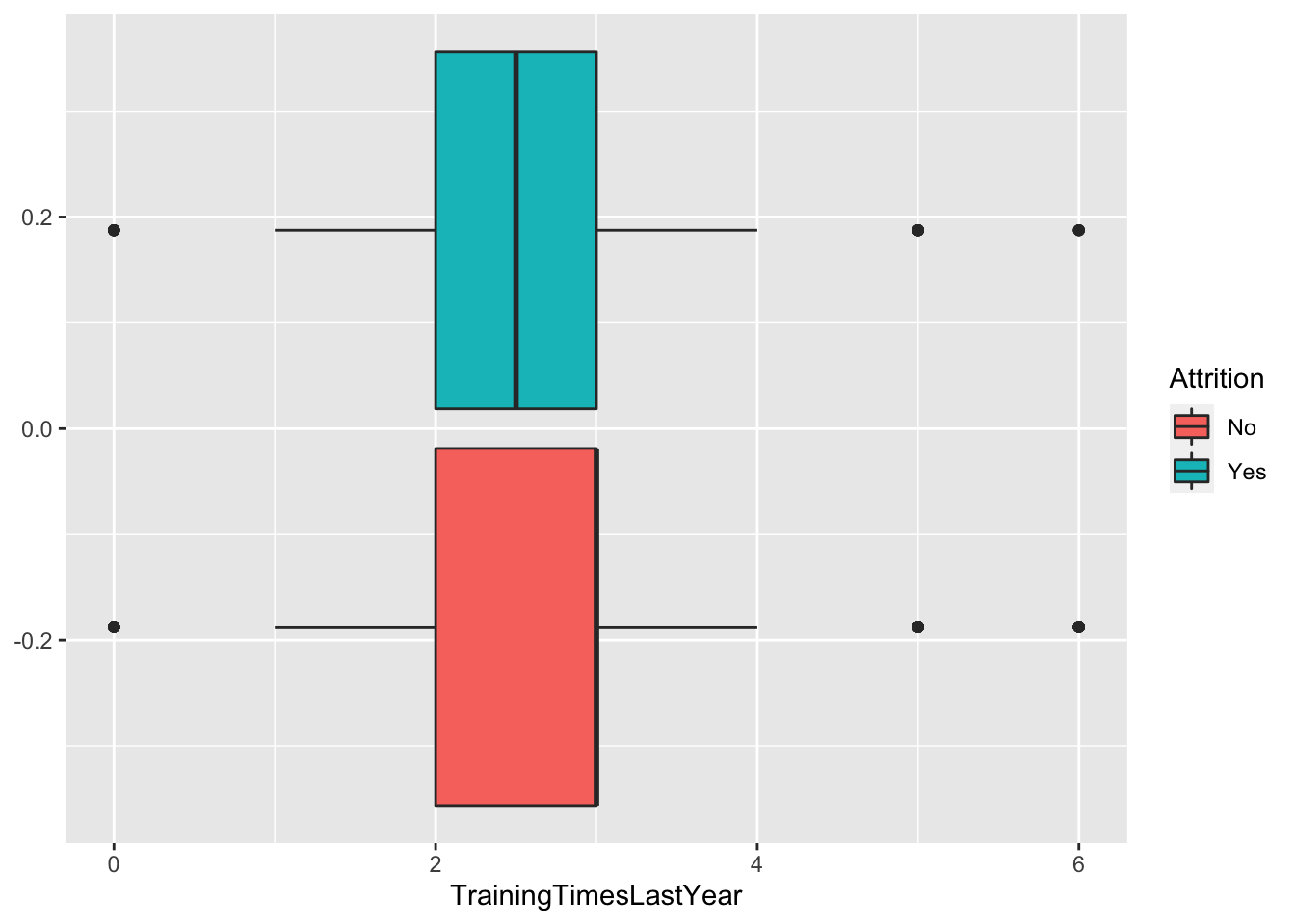

data %>% ggplot(aes(x = WorkLifeBalance, fill = Attrition)) + geom_boxplot()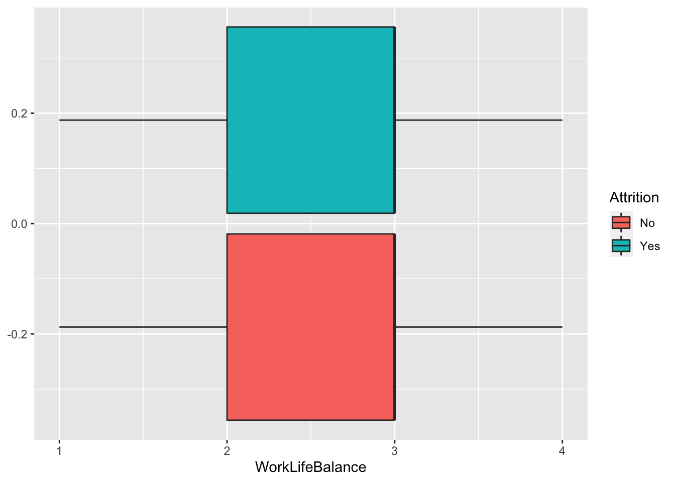

data %>% ggplot(aes(x = YearsAtCompany, fill = Attrition)) + geom_boxplot()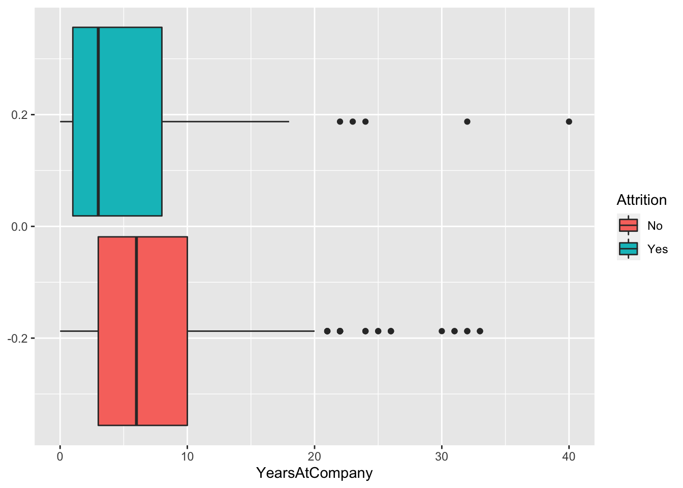

data %>% ggplot(aes(x = YearsInCurrentRole, fill = Attrition)) + geom_boxplot()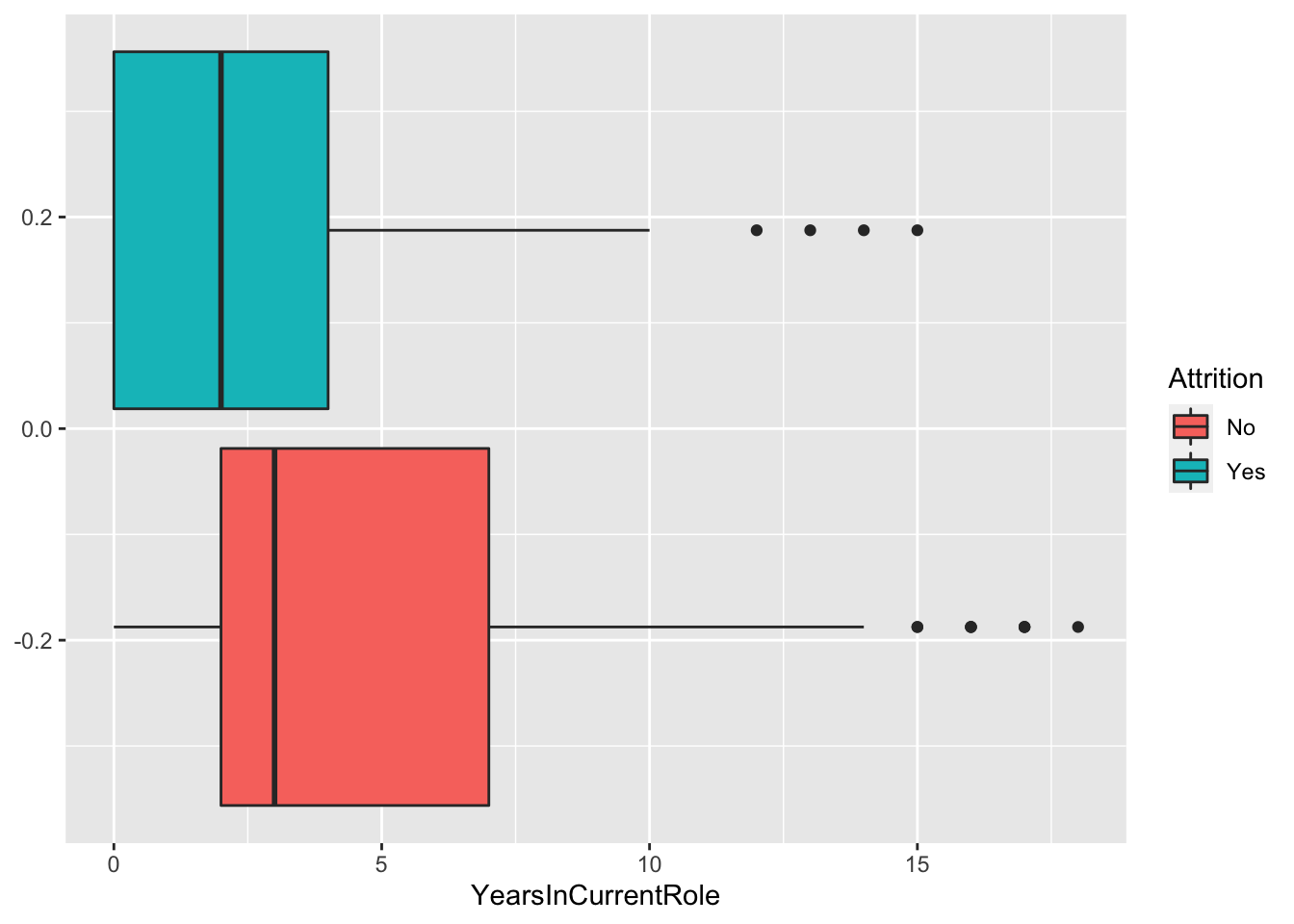

data %>% ggplot(aes(x = YearsSinceLastPromotion, fill = Attrition)) + geom_boxplot()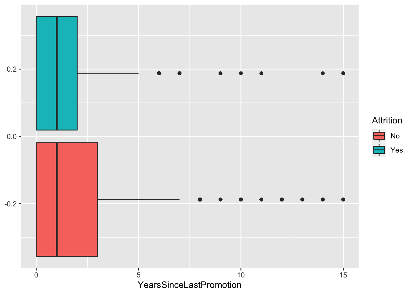

data %>% ggplot(aes(x = YearsWithCurrManager, fill = Attrition)) + geom_boxplot()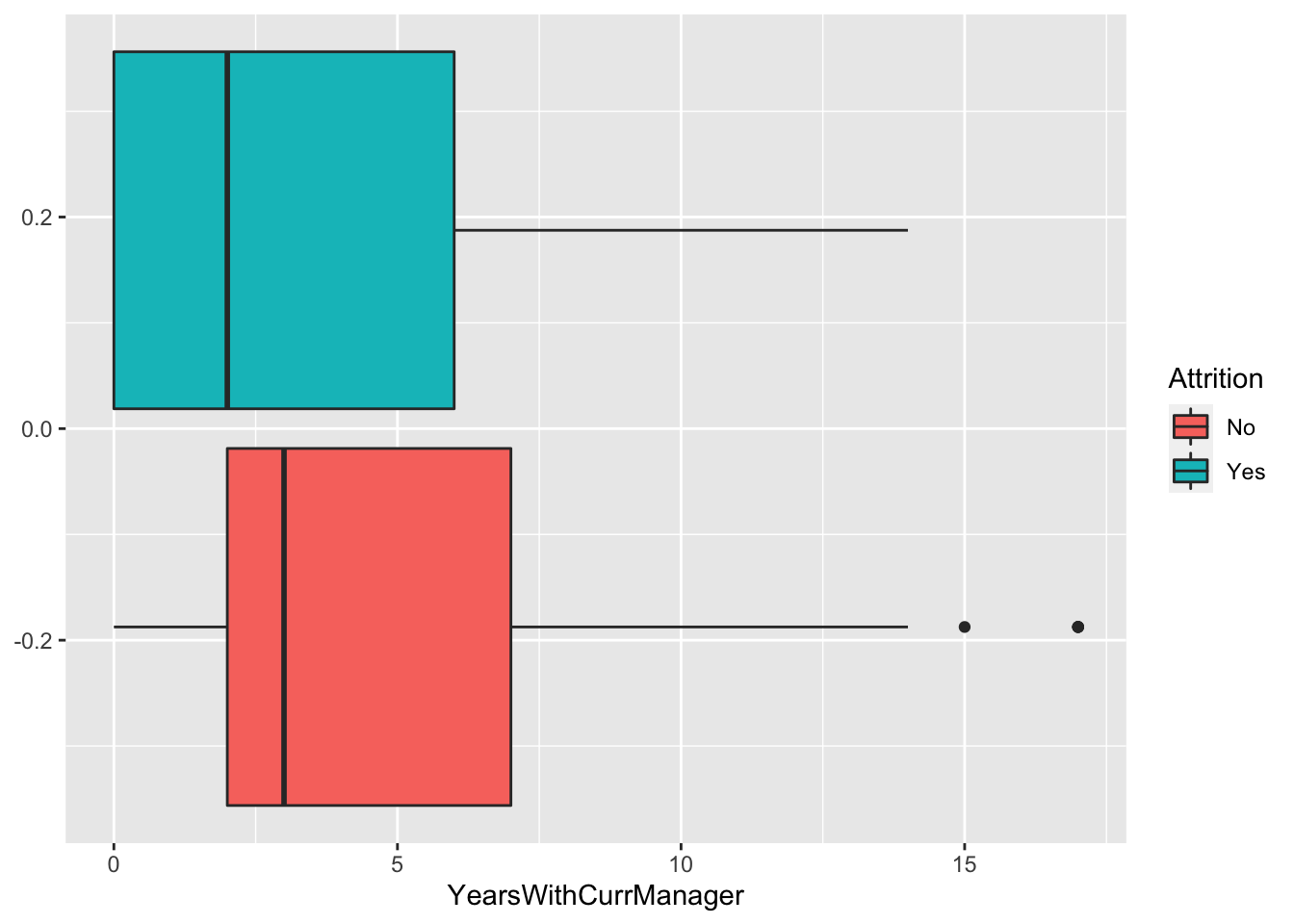

Investigate Distributions of Potentially Relevant Categorical Variables

data %>% ggplot(aes(x = BusinessTravel, fill = Attrition)) + geom_histogram(stat = "count") + facet_wrap(~Attrition)

## Warning: Ignoring unknown parameters: binwidth, bins, pad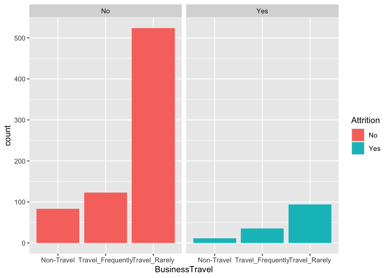

data %>% ggplot(aes(x = EducationField, fill = Attrition)) + geom_histogram(stat = "count") + facet_wrap(~Attrition)

## Warning: Ignoring unknown parameters: binwidth, bins, pad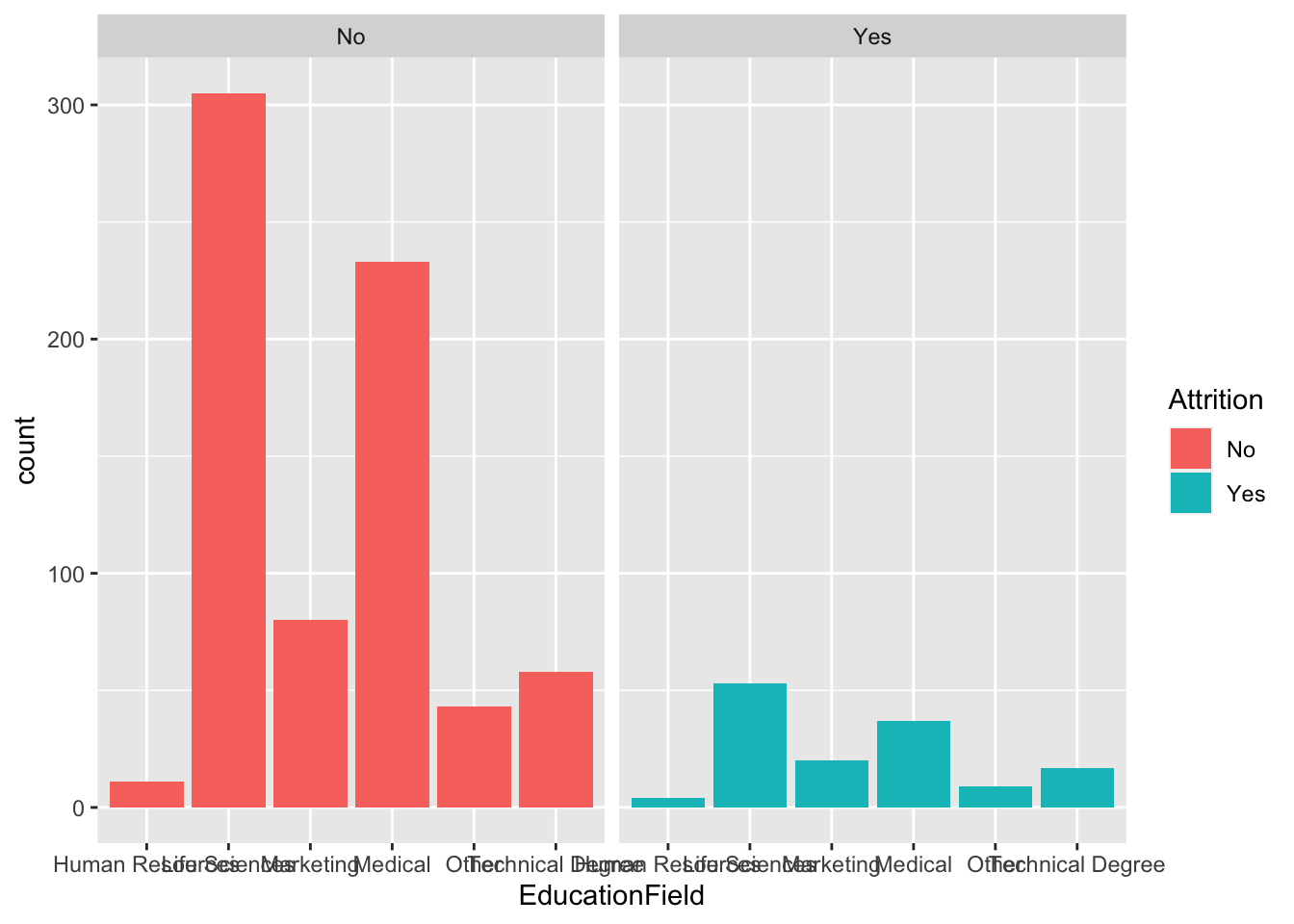

data %>% ggplot(aes(x = Gender, fill = Attrition)) + geom_histogram(stat = "count") + facet_wrap(~Attrition)

## Warning: Ignoring unknown parameters: binwidth, bins, pad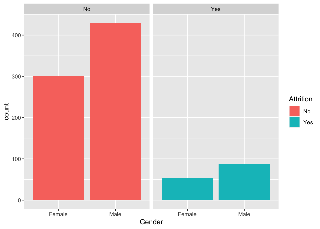

data %>% ggplot(aes(x = MaritalStatus, fill = Attrition)) + geom_histogram(stat = "count") + facet_wrap(~Attrition)

## Warning: Ignoring unknown parameters: binwidth, bins, pad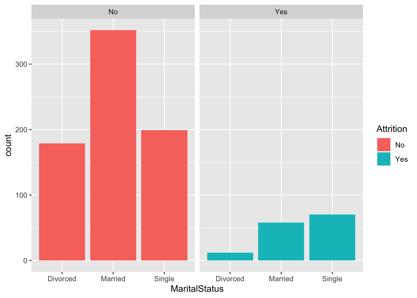

data %>% ggplot(aes(x = Over18, fill = Attrition)) + geom_histogram(stat = "count") + facet_wrap(~Attrition)

## Warning: Ignoring unknown parameters: binwidth, bins, pad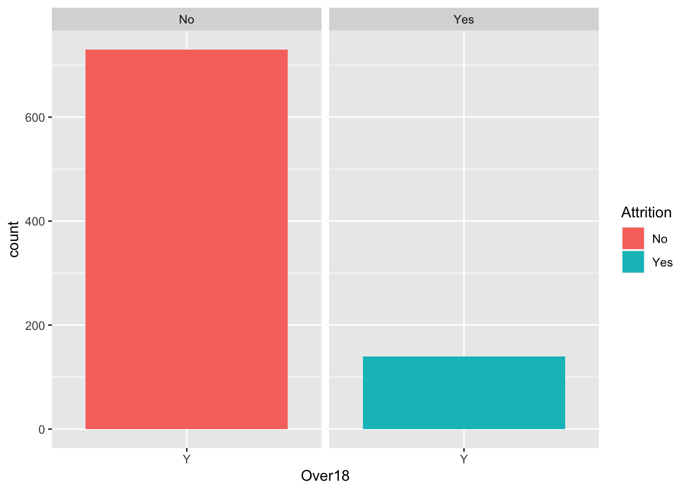

data %>% ggplot(aes(x = JobRole, fill = Attrition)) + geom_histogram(stat = "count") + facet_wrap(~Attrition)

## Warning: Ignoring unknown parameters: binwidth, bins, pad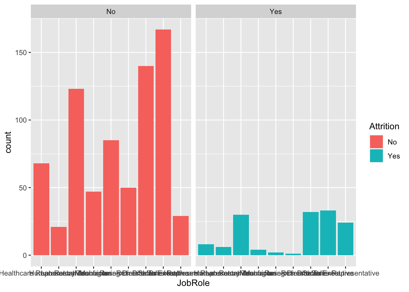

data %>% ggplot(aes(x = OverTime, fill = Attrition)) + geom_histogram(stat = "count") + facet_wrap(~Attrition)

## Warning: Ignoring unknown parameters: binwidth, bins, pad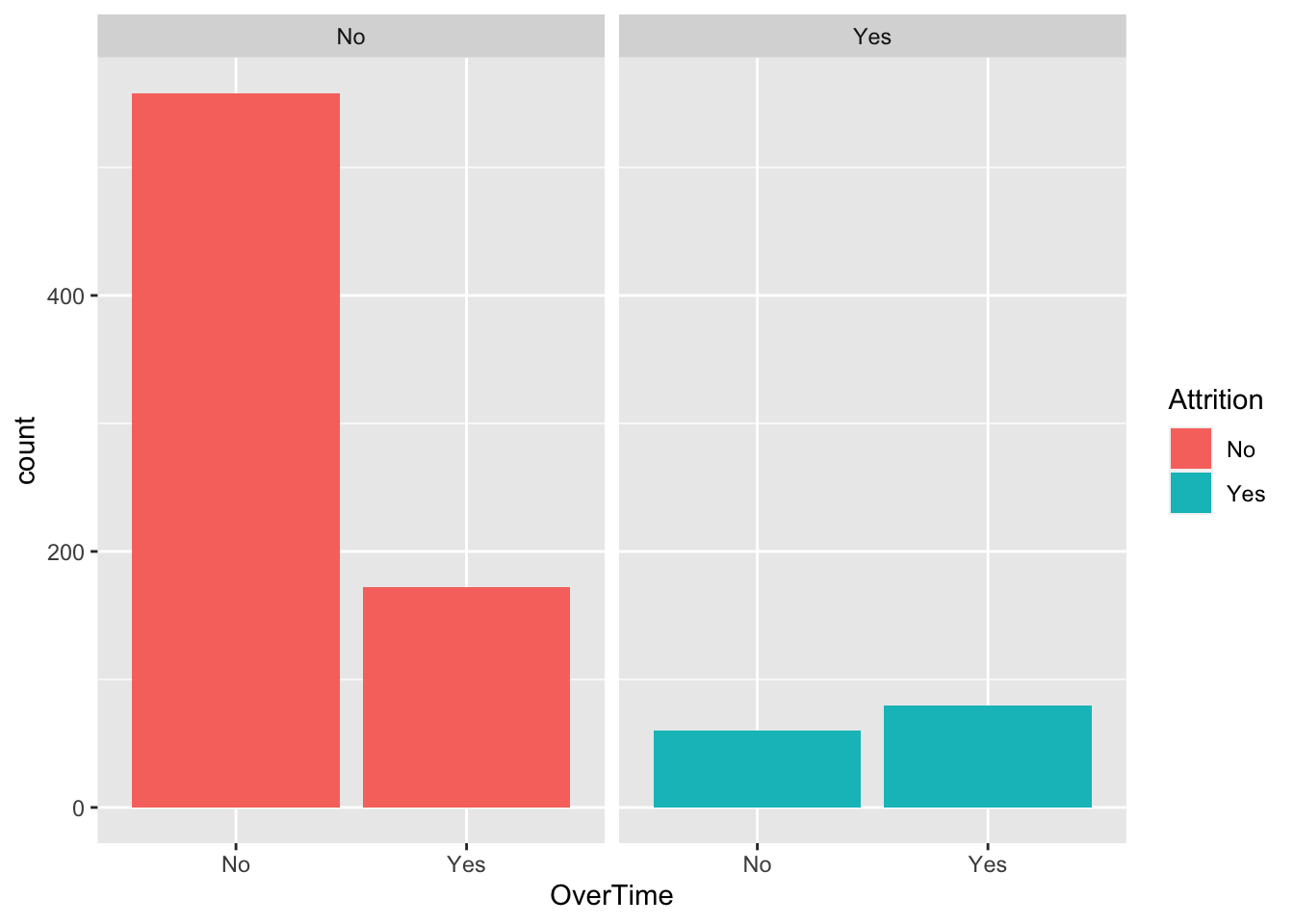

data %>% ggplot(aes(x = Department, fill = Attrition)) + geom_histogram(stat = "count") + facet_wrap(~Attrition)

## Warning: Ignoring unknown parameters: binwidth, bins, pad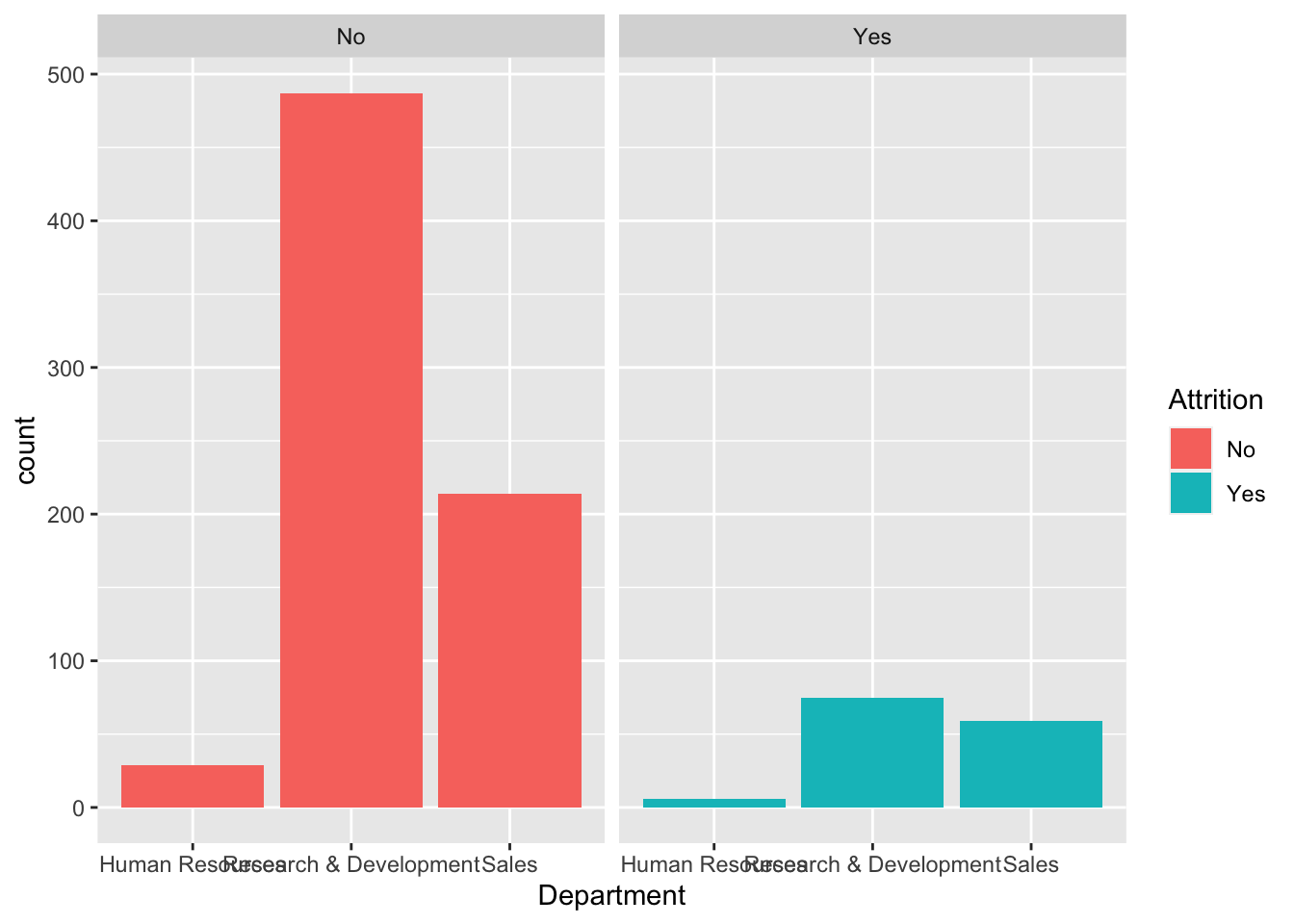

Age Breakdown

#Aggregate Data
age_factor = cut(data$Age, breaks = c(13,19,29,39,49,59,69,79,89), labels = c("Teens", "Twenties", "Thirties", "Forties", "Fifties","Sixties","Seventies","Eighties"))

data = data %>%
  mutate(age_range = age_factor)

data %>%
  group_by(age_range) %>%
  summarize(attrition_count = sum(Attr), Count = n(), perc_attrition = sum(Attr)/n())

## # A tibble: 6 × 4
##   age_range attrition_count Count perc_attrition
##   <fct>               <dbl> <int>          <dbl>
## 1 Teens                   8    13         0.615 
## 2 Twenties               44   172         0.256 
## 3 Thirties               54   381         0.142 
## 4 Forties                21   215         0.0977
## 5 Fifties                13    86         0.151 
## 6 Sixties                 0     3         0

# Plot Aggregated Data - Barplot
data %>%
  group_by(age_range) %>%
  summarize(attrition_count = sum(Attr), Count = n(), perc_attrition = sum(Attr)/n())  %>%
  ggplot(aes(x = age_range, y = perc_attrition, fill = age_range)) +
  geom_bar(stat = "identity") +
  ggtitle("% Attrition by Age") +
  xlab("Age") +
  ylab("% Attrition") +
  theme(legend.position = "none")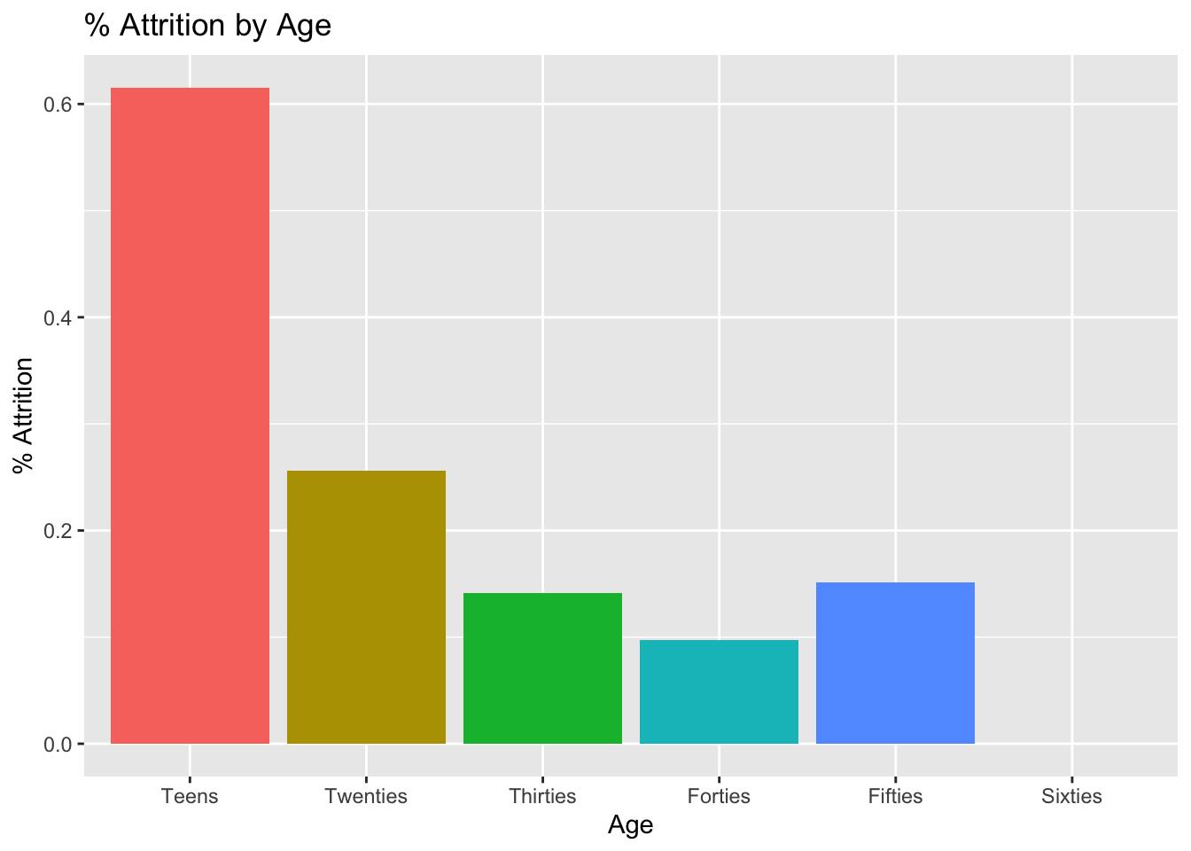

data = data %>% 
  mutate(age_order = case_when(
    grepl("Teens",age_range) ~ 1,
    grepl("Twenties",age_range) ~ 2,
    grepl("Thirties",age_range) ~ 3,
    grepl( "Forties",age_range) ~ 4,
    grepl("Fifties",age_range) ~ 5,
    grepl("Sixties",age_range) ~ 6
  ))


# Scatterplot Comparison

data %>%
  group_by(age_range, age_order) %>%
  summarize(attrition_count = sum(Attr), Count = n(), perc_attrition = sum(Attr)/n())  %>%
  ggplot(aes(x = age_order, y = perc_attrition)) +
  geom_point() +
  geom_smooth(method = "lm") +
  ggtitle("% Attrition by Age") +
  xlab("Age Rank") +
  ylab("% Attrition") +
  theme(legend.position = "none")

## `summarise()` has grouped output by 'age_range'. You can override using the `.groups` argument.

## `geom_smooth()` using formula 'y ~ x'

Satisfaction Score Creation

data = data %>%
  mutate(OverallSatisfaction = (JobSatisfaction+EnvironmentSatisfaction+WorkLifeBalance+RelationshipSatisfaction)/4)

data %>%
  group_by(OverallSatisfaction) %>%
   summarize(perc_attrition = sum(Attr)/n()) %>%
  ggplot(aes(x = OverallSatisfaction, perc_attrition)) +
  geom_point() +
  geom_smooth(method = "lm") +
  ylim(0,1)

## `geom_smooth()` using formula 'y ~ x'

## Warning: Removed 10 rows containing missing values (geom_smooth).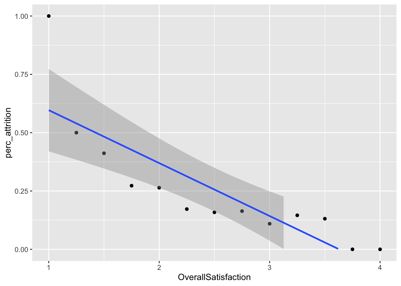

Involvement Score Creation

data = data %>%
  mutate(Involvement = (JobInvolvement+TrainingTimesLastYear+StockOptionLevel)/3)

data %>%
  group_by(Involvement) %>%
  summarize(perc_attrition = sum(Attr)/n()) %>%
  ggplot(aes(x = Involvement, y = perc_attrition)) +
  geom_point() +
  geom_smooth(method = "lm")

## `geom_smooth()` using formula 'y ~ x'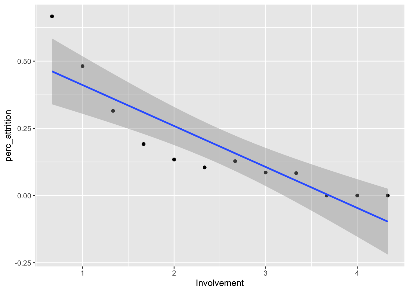

Percent Attrition by key Discrete attributes

# Years by perc attrition
data %>%
  group_by(YearsAtCompany) %>%
  summarize(perc_attrition = sum(Attr)/n()) %>%
  ggplot(aes(x = YearsAtCompany, y = perc_attrition)) +
  geom_point()

data %>%
  group_by(YearsAtCompany) %>%
 summarize(perc_attrition = sum(Attr)/n()) %>%
  ggplot(aes(x = YearsAtCompany, y = perc_attrition)) +
  geom_point()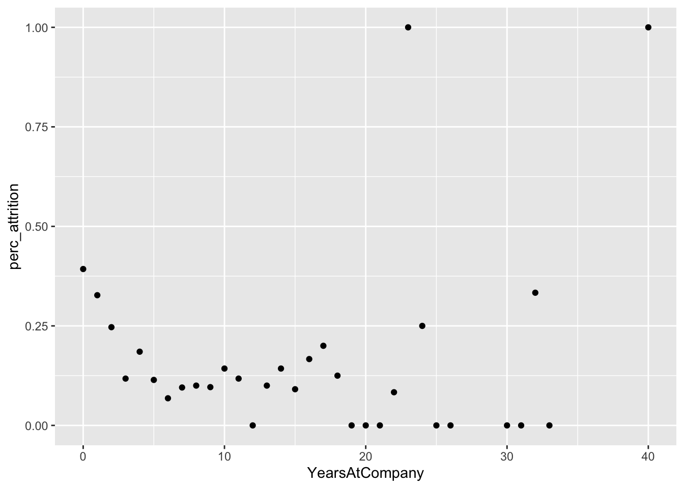

# Distance by perc Attrition
data %>%
  group_by(DistanceFromHome) %>%
 summarize(perc_attrition = sum(Attr)/n()) %>%
  ggplot(aes(x = DistanceFromHome, y = perc_attrition)) +
  geom_point()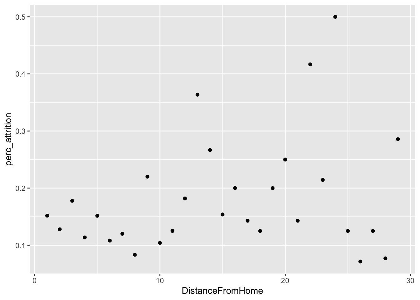

# Total Working Years by Attrition
data %>%
  group_by(TotalWorkingYears) %>%
 summarize(perc_attrition = sum(Attr)/n()) %>%
  ggplot(aes(x = TotalWorkingYears, y = perc_attrition)) +
  geom_point()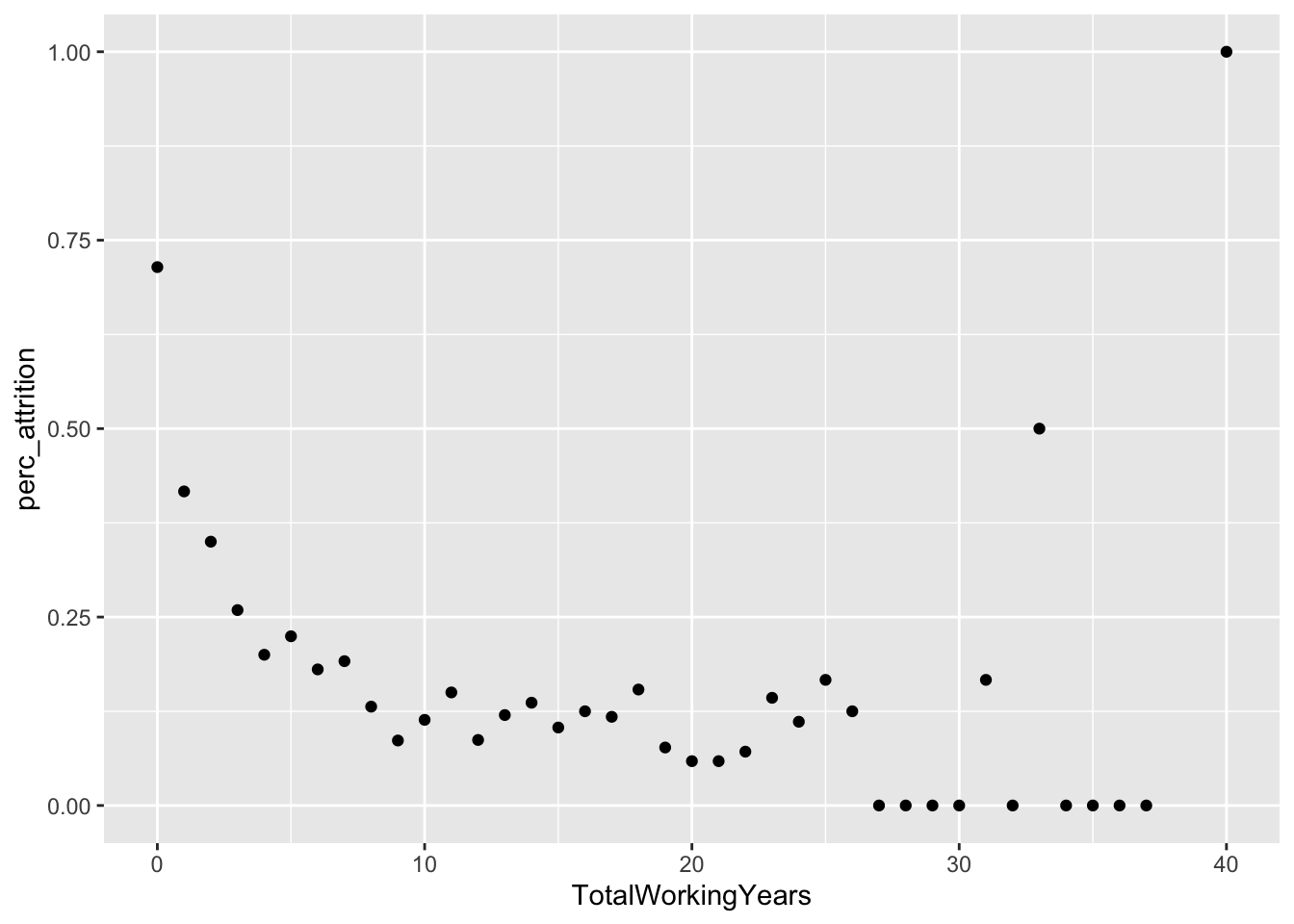

Percent Attrition by key Categorical attributes

# Higher chance of attrition for teen males
data %>%
  group_by(age_range, Gender) %>%
  summarize(perc_attrition = sum(Attr)/n()) %>%
  ggplot(aes(x = age_range, y = Gender, fill = perc_attrition)) + 
  geom_tile()

## `summarise()` has grouped output by 'age_range'. You can override using the `.groups` argument.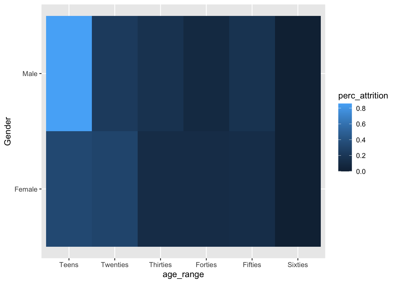

# Higher chance of attrition for sales representatives
data %>%
  group_by(Department, JobRole) %>%
  summarize(perc_attrition = sum(Attr)/n()) %>%
  ggplot(aes(x = Department, y = JobRole, fill = perc_attrition)) + 
  geom_tile()

## `summarise()` has grouped output by 'Department'. You can override using the `.groups` argument.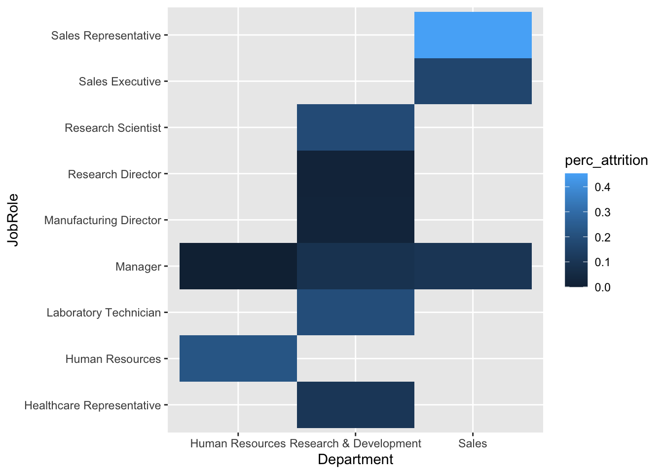

# Higher chance of attrition for single individuals with a technical degree
data %>%
  group_by(MaritalStatus, EducationField) %>%
  summarize(perc_attrition = sum(Attr)/n()) %>%
  ggplot(aes(x = MaritalStatus, y = EducationField, fill = perc_attrition)) + 
  geom_tile()

## `summarise()` has grouped output by 'MaritalStatus'. You can override using the `.groups` argument.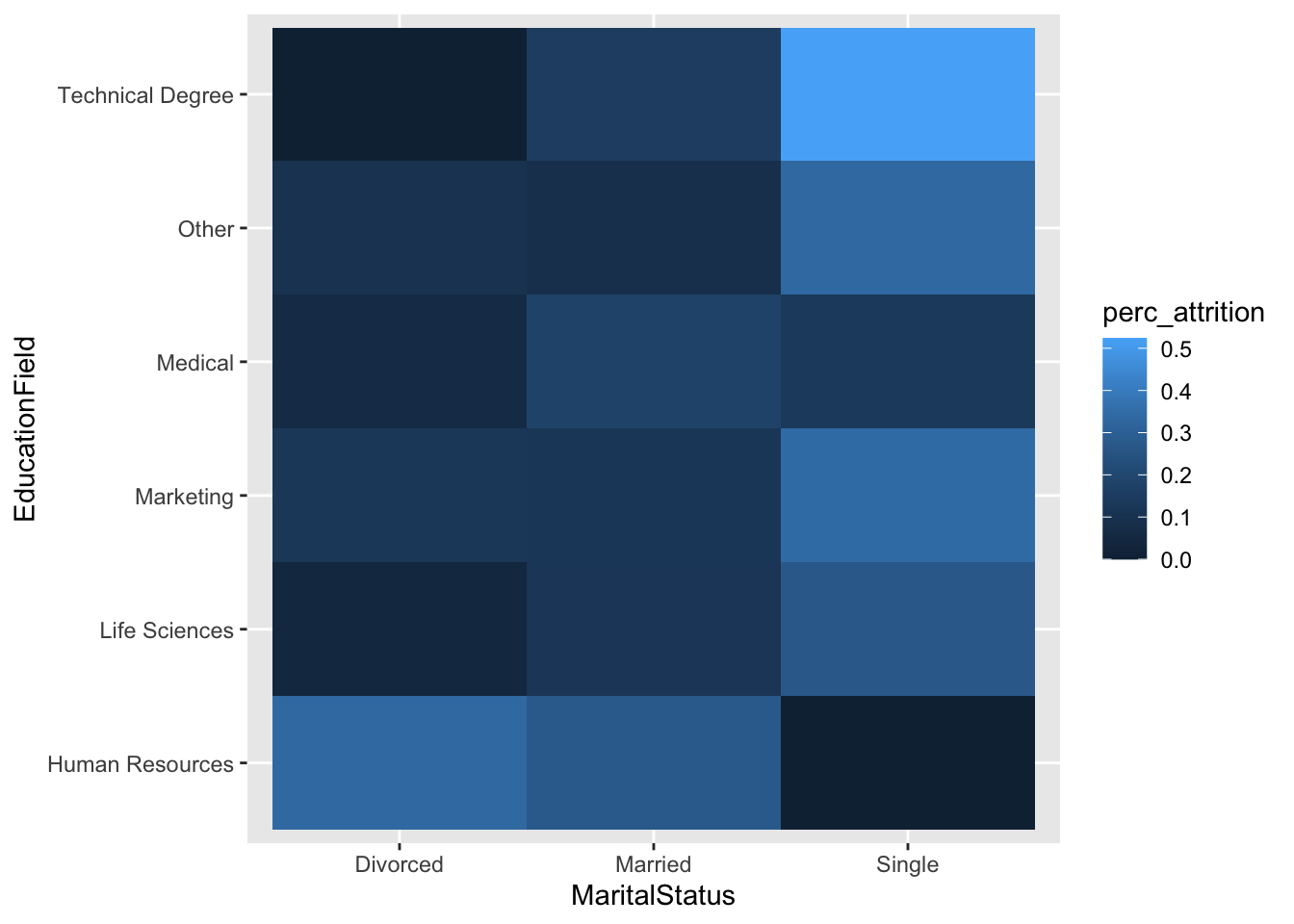

Education Field Attrition

#Aggregate Data

data %>%
  group_by(EducationField) %>%
  summarize(attrition_count = sum(Attr), Count = n(), perc_attrition = sum(Attr)/n())

## # A tibble: 6 × 4
##   EducationField   attrition_count Count perc_attrition
##   <chr>                      <dbl> <int>          <dbl>
## 1 Human Resources                4    15          0.267
## 2 Life Sciences                 53   358          0.148
## 3 Marketing                     20   100          0.2  
## 4 Medical                       37   270          0.137
## 5 Other                          9    52          0.173
## 6 Technical Degree              17    75          0.227

# Plot Aggregated Data
data %>%
  group_by(EducationField) %>%
  summarize(attrition_count = sum(Attr), Count = n(), perc_attrition = sum(Attr)/n())  %>%
  ggplot(aes(x = reorder(EducationField, perc_attrition), y = perc_attrition, fill = EducationField)) +
  geom_bar(stat = "identity") +
  ggtitle("% Attrition by Education Field") +
  xlab("Education Field") +
  ylab("% Attrition") +
  theme(legend.position = "none")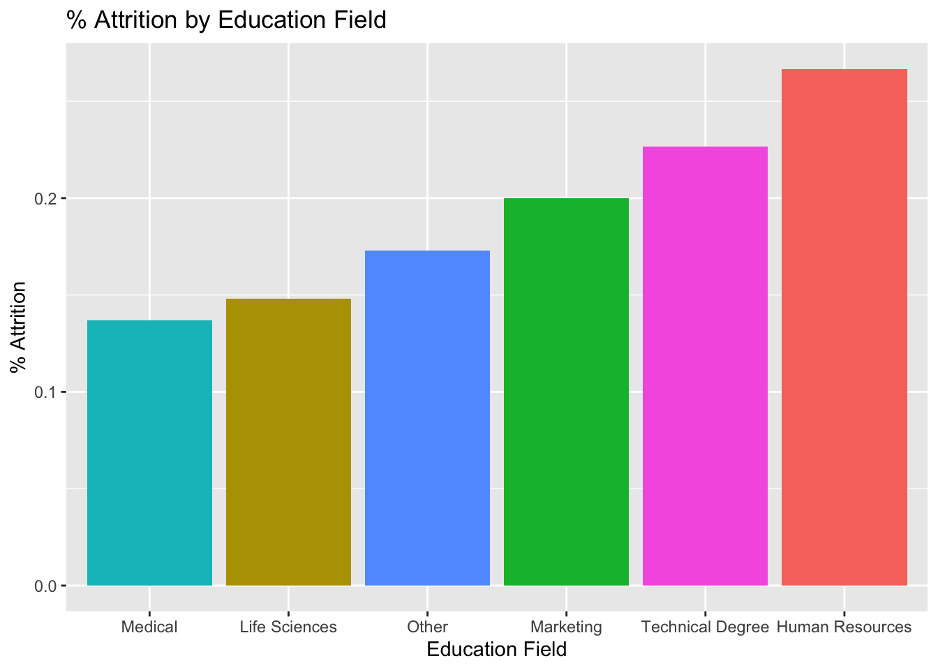

Education Field Satisfaction

#Aggregate Data

data %>%
  group_by(EducationField) %>%
  summarize(Count = n(), avg_satisfaction = sum(JobSatisfaction)/n())

## # A tibble: 6 × 3
##   EducationField   Count avg_satisfaction
##   <chr>            <int>            <dbl>
## 1 Human Resources     15             2.47
## 2 Life Sciences      358             2.74
## 3 Marketing          100             2.68
## 4 Medical            270             2.71
## 5 Other               52             2.75
## 6 Technical Degree    75             2.6

# Plot Aggregated Data
data %>%
  group_by(EducationField) %>%
  summarize(Count = n(), avg_satisfaction = sum(JobSatisfaction)/n()) %>%
  ggplot(aes(x = reorder(EducationField, avg_satisfaction), y = avg_satisfaction, fill = EducationField)) +
  geom_bar(stat = "identity") +
  ggtitle("Avg Satisfaction by Education Field") +
  xlab("Education Field") +
  ylab("Avg Satisfaction") +
  coord_cartesian(ylim=c(2.4,2.75)) +
  theme(legend.position = "none")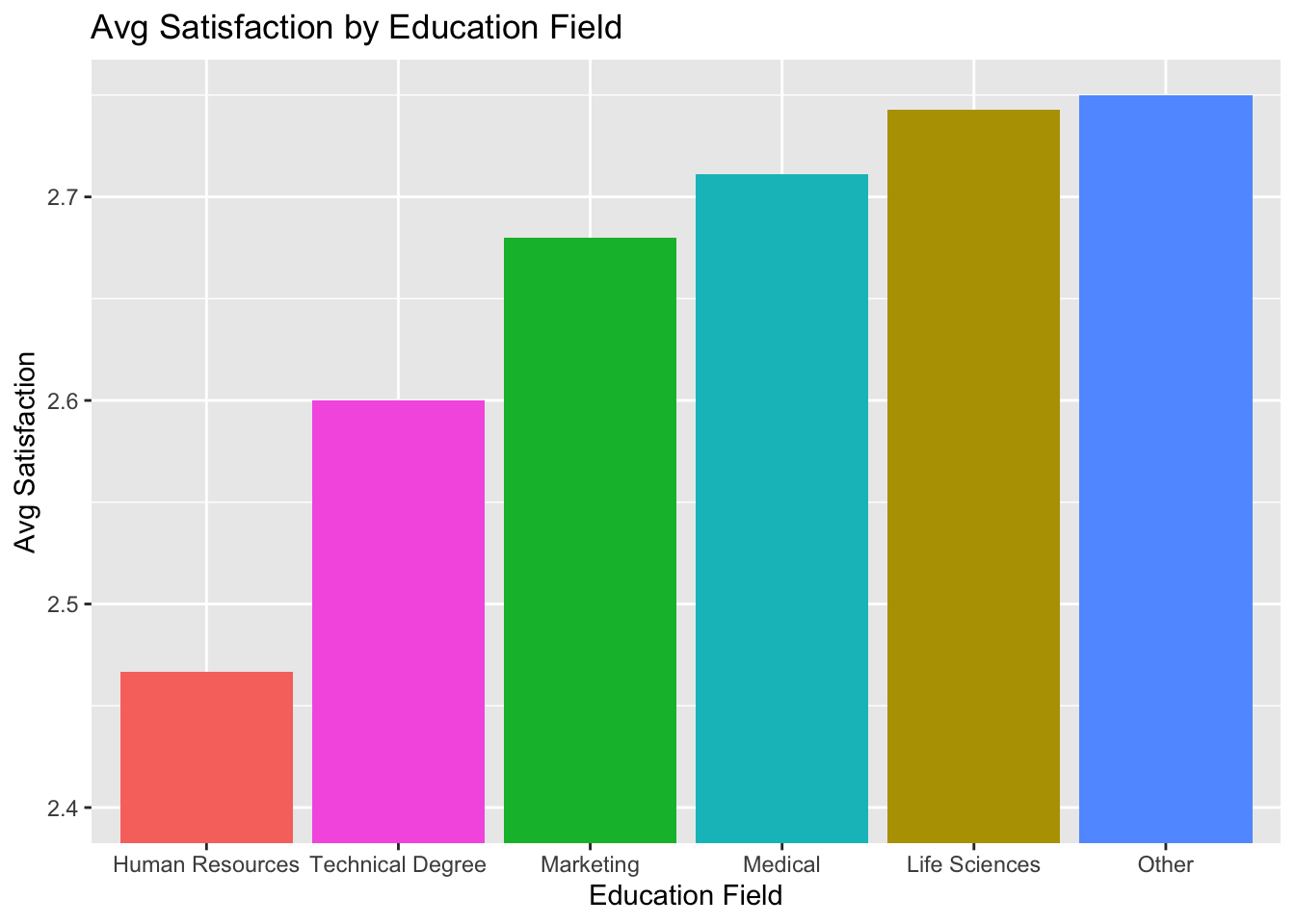

Position Attrition

#Aggregate Data
data %>%
  group_by(JobRole) %>%
  summarize(attrition_count = sum(Attr), Count = n(), perc_attrition = sum(Attr)/n())

## # A tibble: 9 × 4
##   JobRole                   attrition_count Count perc_attrition
##   <chr>                               <dbl> <int>          <dbl>
## 1 Healthcare Representative               8    76         0.105 
## 2 Human Resources                         6    27         0.222 
## 3 Laboratory Technician                  30   153         0.196 
## 4 Manager                                 4    51         0.0784
## 5 Manufacturing Director                  2    87         0.0230
## 6 Research Director                       1    51         0.0196
## 7 Research Scientist                     32   172         0.186 
## 8 Sales Executive                        33   200         0.165 
## 9 Sales Representative                   24    53         0.453

# Plot Aggregated Data

data %>%
  group_by(JobRole) %>%
  summarize(attrition_count = sum(Attr), Count = n(), perc_attrition = sum(Attr)/n())  %>%
  ggplot(aes(x = reorder(JobRole, perc_attrition), y = perc_attrition, fill = JobRole)) +
  geom_bar(stat = "identity") +
  ggtitle("% Attrition by Position") +
  xlab("Position") +
  ylab("% Attrition") +
  theme(legend.position = "none") +
  theme(axis.text.x = element_text(angle = 50, 
                                   vjust = 1, 
                                   hjust = 1,
                                   size = 8))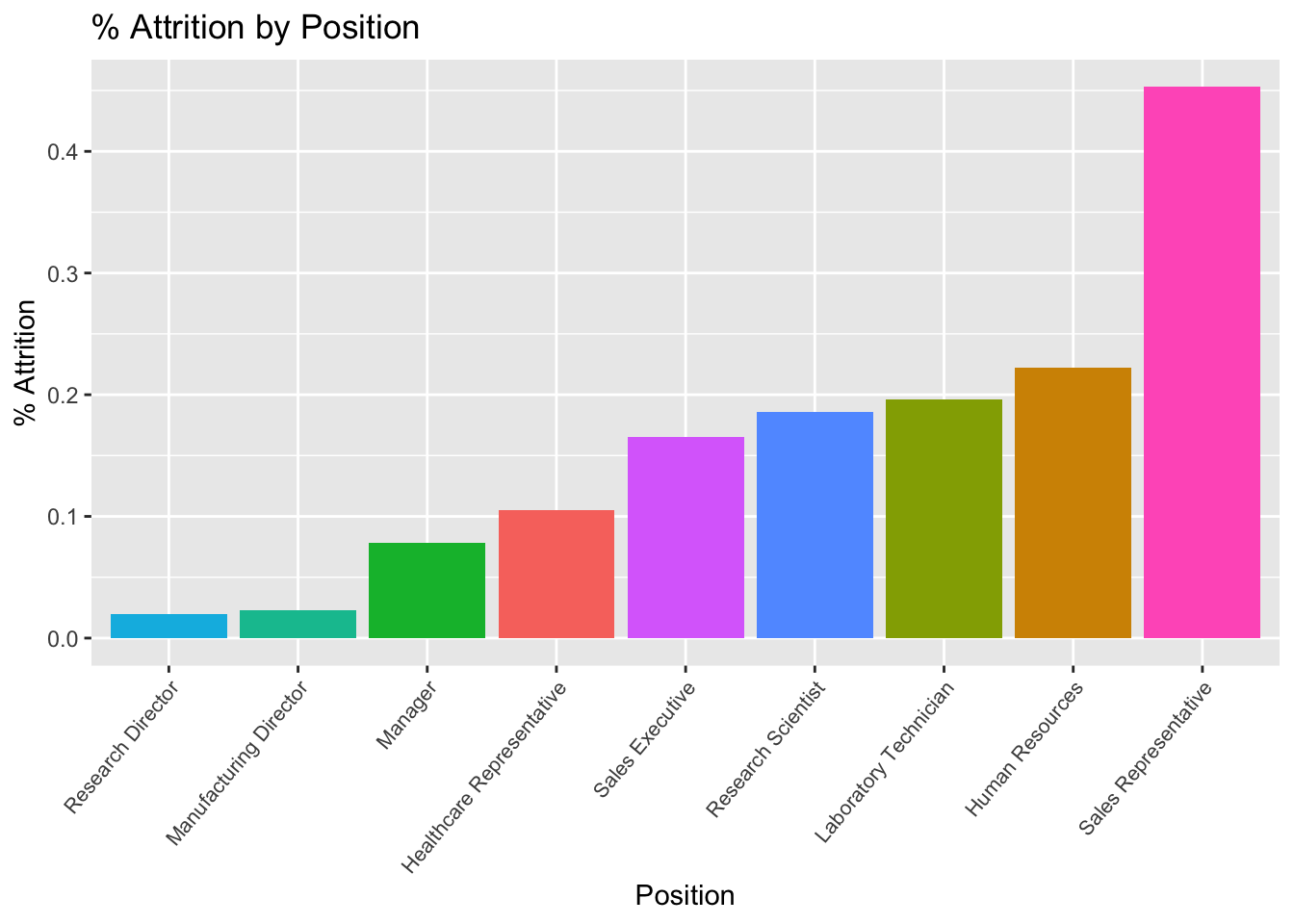

Position Avg Satisfaction

#Aggregate Data
data %>%
  group_by(JobRole) %>%
  summarize(Count = n(),avg_satisfaction = sum(JobSatisfaction)/n())

## # A tibble: 9 × 3
##   JobRole                   Count avg_satisfaction
##   <chr>                     <int>            <dbl>
## 1 Healthcare Representative    76             2.83
## 2 Human Resources              27             2.56
## 3 Laboratory Technician       153             2.69
## 4 Manager                      51             2.51
## 5 Manufacturing Director       87             2.72
## 6 Research Director            51             2.49
## 7 Research Scientist          172             2.80
## 8 Sales Executive             200             2.72
## 9 Sales Representative         53             2.70

# Plot Aggregated Data

data %>%
  group_by(JobRole) %>%
  summarize(Count = n(),avg_satisfaction = sum(JobSatisfaction)/n())   %>%
  ggplot(aes(x = reorder(JobRole,avg_satisfaction), y = avg_satisfaction, fill = JobRole)) +
  geom_bar(stat = "identity") +
  ggtitle("Avg Satisfaction by Position") +
  xlab("Position") +
  ylab("Avg Satisfaction") +
  theme(legend.position = "none") +
  coord_cartesian(ylim=c(2.4,2.85)) +
  theme(axis.text.x = element_text(angle = 50, 
                                   vjust = 1, 
                                   hjust = 1,
                                   size = 8))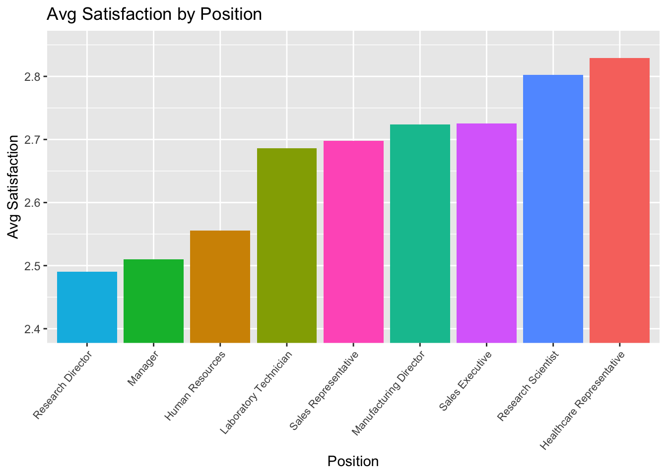

Gender / Age Attrition

#Aggregate Data
age_data = data %>%
  group_by(Gender, age_range) %>%
  summarize(attrition_count = sum(Attr), Count = n(), perc_attrition = sum(Attr)/n())

## `summarise()` has grouped output by 'Gender'. You can override using the `.groups` argument.

age_gender = data.frame(paste(age_data$Gender, age_data$age_range))
colnames(age_gender) = "age_gender"
age_data = cbind(age_data, age_gender)
age_data$age_gender = factor(age_data$age_gender)

age_data = age_data %>% 
  mutate(order = case_when(
    grepl("Teens",age_range) ~ 1,
    grepl("Twenties",age_range) ~ 2,
    grepl("Thirties",age_range) ~ 3,
    grepl( "Forties",age_range) ~ 4,
    grepl("Fifties",age_range) ~ 5,
    grepl("Sixties",age_range) ~ 6
  ))

# Plot Aggregated Data

age_data %>%
  ggplot(aes(x = reorder(age_gender,order), y = perc_attrition, fill = Gender)) +
  geom_bar(stat = "identity") +
  ggtitle("% Attrition by Age and Gender") +
  xlab("Age / Gender") +
  ylab("% Attrition") +
  theme(legend.position = "none") +
  theme(axis.text.x = element_text(angle = 50, 
                                   vjust = 1, 
                                   hjust = 1,
                                   size = 8))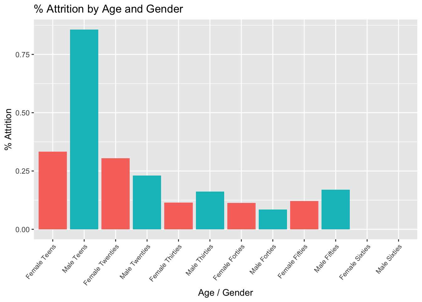

Gender / Age Avg Satisfaction

#Aggregate Data
age_data = data %>%
  group_by(Gender, age_range) %>%
  summarize(Count = n(), avg_satisfaction = sum(JobSatisfaction)/n())

## `summarise()` has grouped output by 'Gender'. You can override using the `.groups` argument.

age_gender = data.frame(paste(age_data$Gender, age_data$age_range))
colnames(age_gender) = "age_gender"
age_data = cbind(age_data, age_gender)
age_data$age_gender = factor(age_data$age_gender)

age_data = age_data %>% 
  mutate(order = case_when(
    grepl("Teens",age_range) ~ 1,
    grepl("Twenties",age_range) ~ 2,
    grepl("Thirties",age_range) ~ 3,
    grepl( "Forties",age_range) ~ 4,
    grepl("Fifties",age_range) ~ 5,
    grepl("Sixties",age_range) ~ 6
  ))

# Plot Aggregated Data

age_data %>%
  ggplot(aes(x = reorder(age_gender,order), y = avg_satisfaction, fill = Gender)) +
  geom_bar(stat = "identity") +
  ggtitle("Avg Satisfaction by Age and Gender") +
  xlab("Age / Gender") +
  ylab("Avg Satisfaction") +
  theme(legend.position = "none") +
  coord_cartesian(ylim=c(2.4,3.2)) +
  theme(axis.text.x = element_text(angle = 50, 
                                   vjust = 1, 
                                   hjust = 1,
                                   size = 8))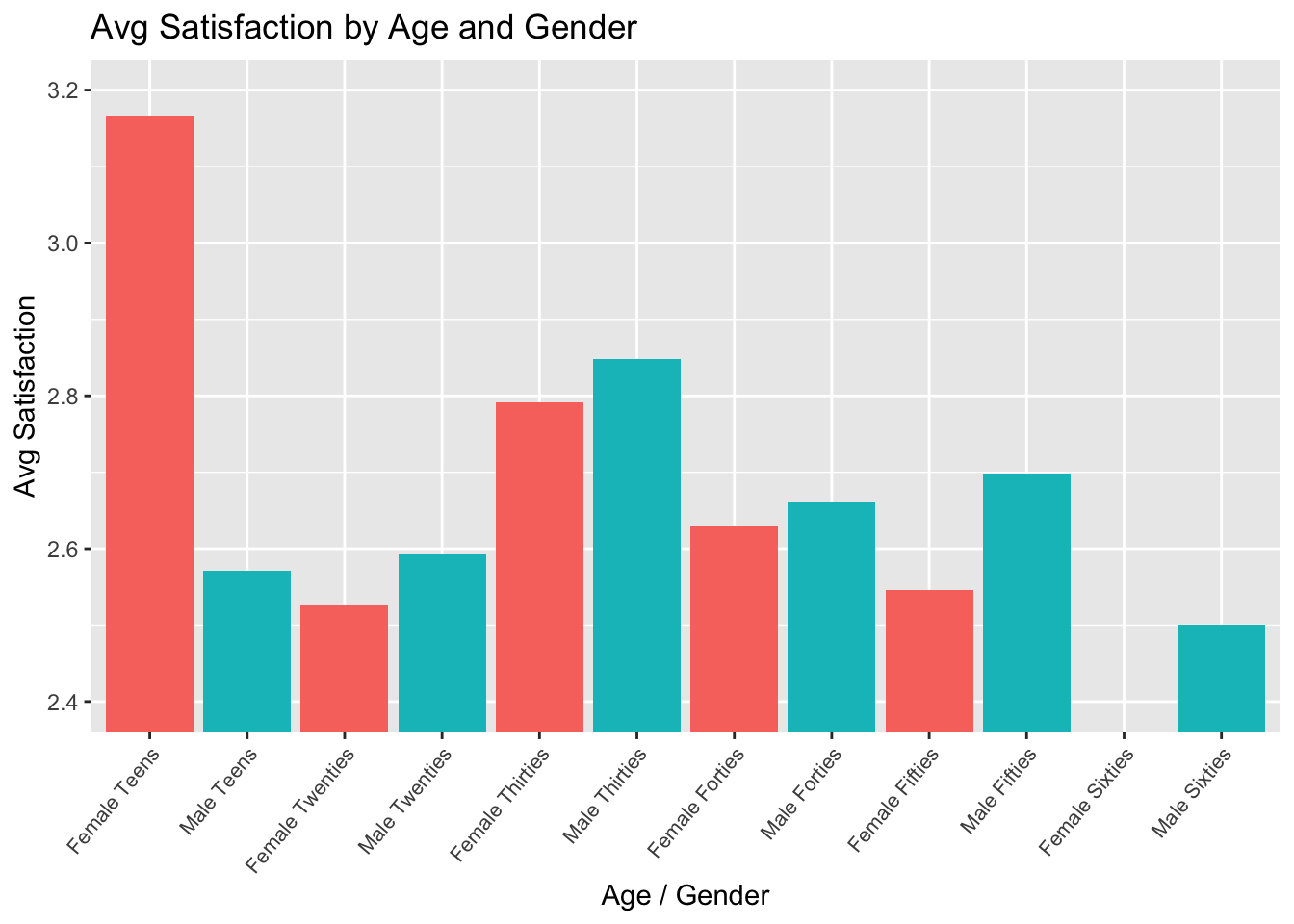

Gender / Age / Marital Status Attrition

#Aggregate Data
age_data = data %>%
  group_by(MaritalStatus, Gender, age_range) %>%
  summarize(attrition_count = sum(Attr), Count = n(), perc_attrition = sum(Attr)/n())

## `summarise()` has grouped output by 'MaritalStatus', 'Gender'. You can override using the `.groups` argument.

age_gender = data.frame(paste(age_data$Gender, age_data$MaritalStatus, age_data$age_range))
colnames(age_gender) = "age_gender_marital"
age_data = cbind(age_data, age_gender)
age_data$age_gender_marital = factor(age_data$age_gender_marital)

age_data = age_data %>% 
  mutate(order = case_when(
    grepl("Teens",age_range) ~ 1,
    grepl("Twenties",age_range) ~ 2,
    grepl("Thirties",age_range) ~ 3,
    grepl( "Forties",age_range) ~ 4,
    grepl("Fifties",age_range) ~ 5,
    grepl("Sixties",age_range) ~ 6
  ))

# Plot Aggregated Data

age_data %>%
  ggplot(aes(x = reorder(age_gender_marital,order), y = perc_attrition, fill = Gender)) + 
  geom_bar(stat = "identity") +
  ggtitle("% Attrition by Age, Gender, and Marital Status") +
  xlab("Age / Gender / Marital Status") +
  ylab("% Attrition") +
  theme(legend.position = "none") +
  theme(axis.text.x = element_text(angle = 50, 
                                   vjust = 1, 
                                   hjust = 1,
                                   size = 8))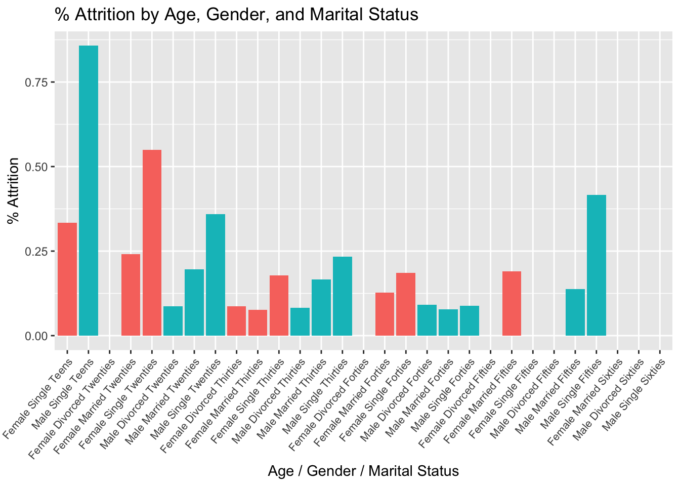

Investigating Relationship betweeen Income, Satisfaction, and Job Level

roledata = data %>%
  select(JobRole,JobLevel,OverallSatisfaction,TrainingTimesLastYear,MonthlyIncome) %>%
  mutate(RoleLevel = paste(JobRole, " Level: ", JobLevel))

graph_roledata = roledata %>%
  group_by(RoleLevel) %>%
  summarize(AvgIncome = sum(MonthlyIncome)/n(), AvgTraining = sum(TrainingTimesLastYear)/n(), AvgSatisfaction = sum(OverallSatisfaction)/n()) 

graph_roledata %>%
  ggplot(aes(x = RoleLevel, y = AvgIncome, fill = AvgSatisfaction)) +
  geom_bar(stat = "identity") +
  theme(axis.text.x = element_text(angle = 90, 
                                   vjust = 1, 
                                   hjust = 1,
                                   size = 8)) +
  ggtitle("Monthly Income by Role / Level") +
  ylab("Avg Monthly Income") +
  xlab("Role / Level")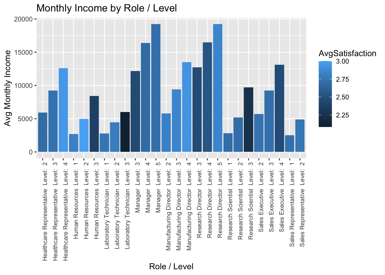

graph_roledata %>%
  ggplot(aes(x = reorder(RoleLevel, AvgSatisfaction), y = AvgSatisfaction)) +
  geom_bar(stat = "identity", fill = "darkslategray3") +
  theme(axis.text.x = element_text(angle = 70, 
                                   vjust = 1, 
                                   hjust = 1,
                                   size = 8)) +
  ggtitle("Satisfaction by Role / Level") +
  ylab("Avg Satisfaction") +
  xlab("Role / Level")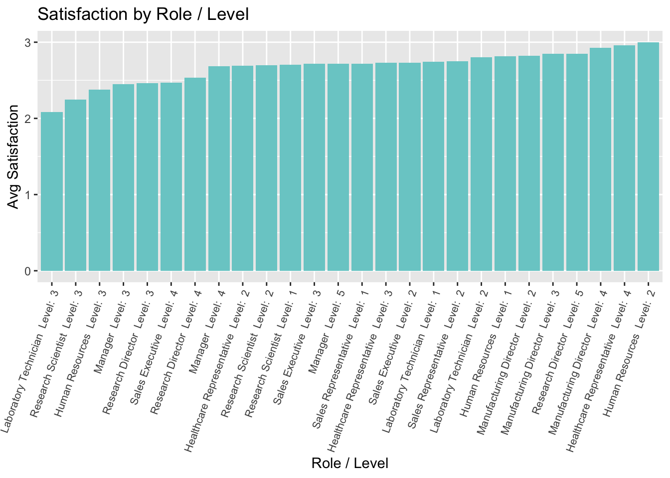

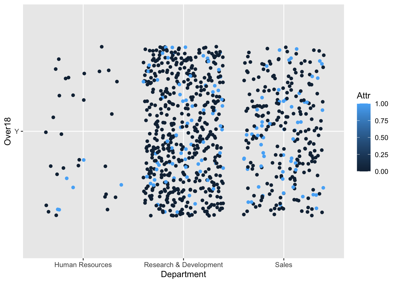
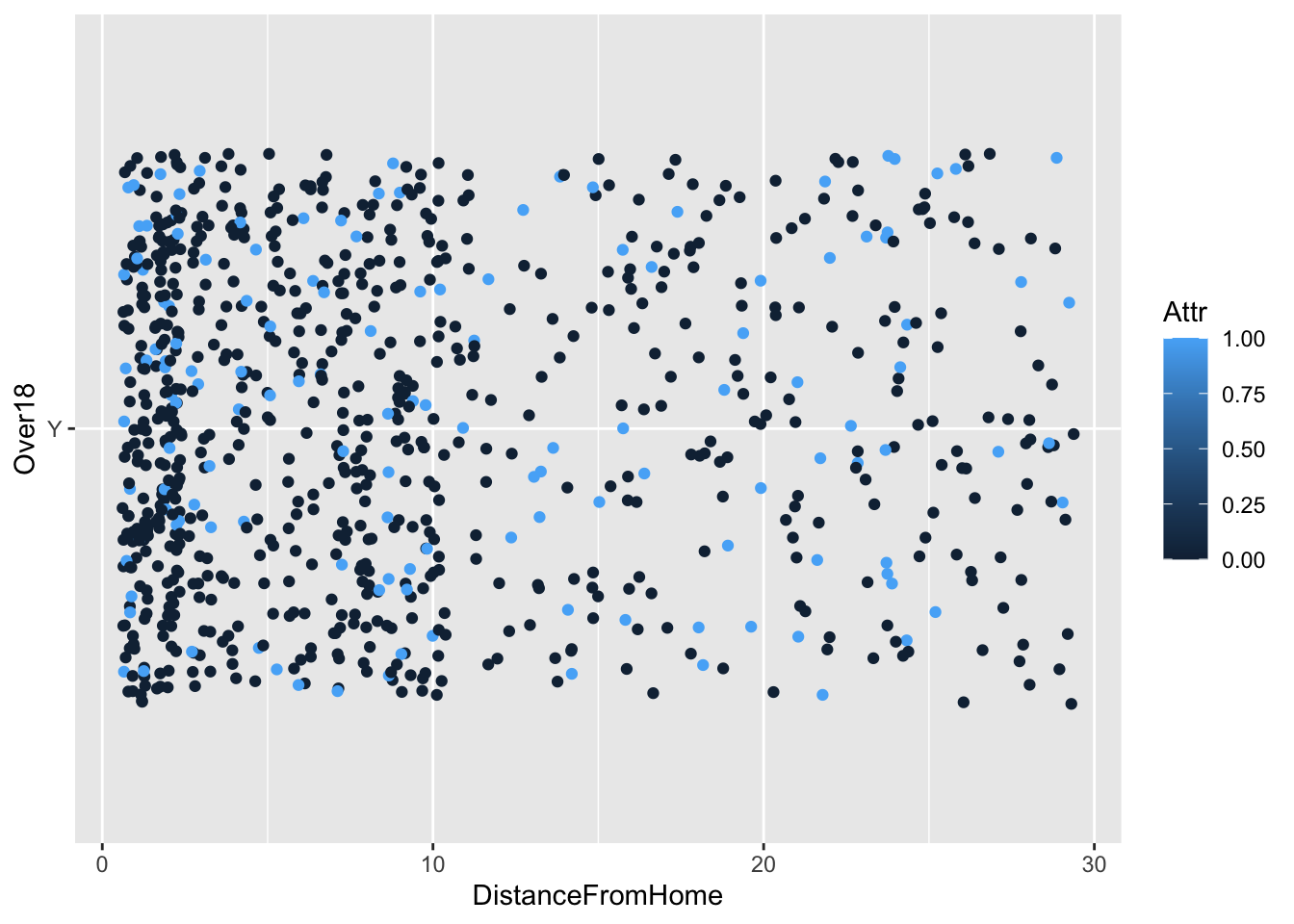
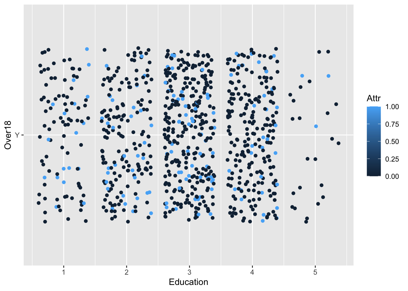
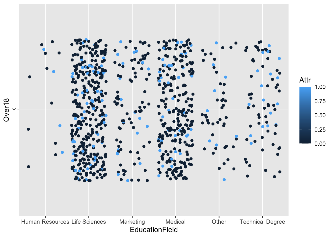
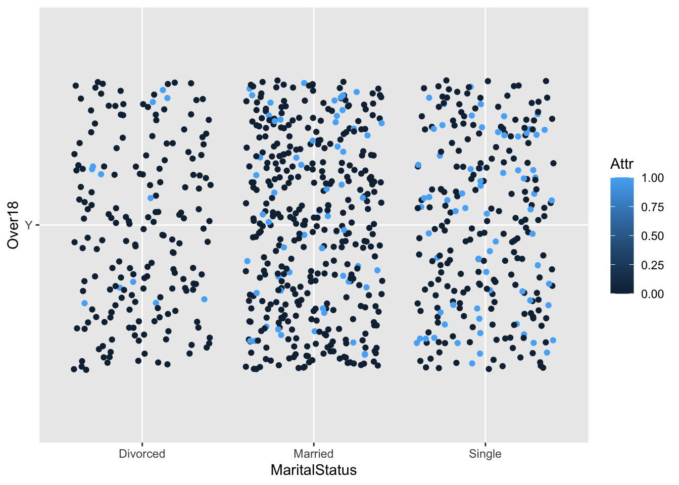
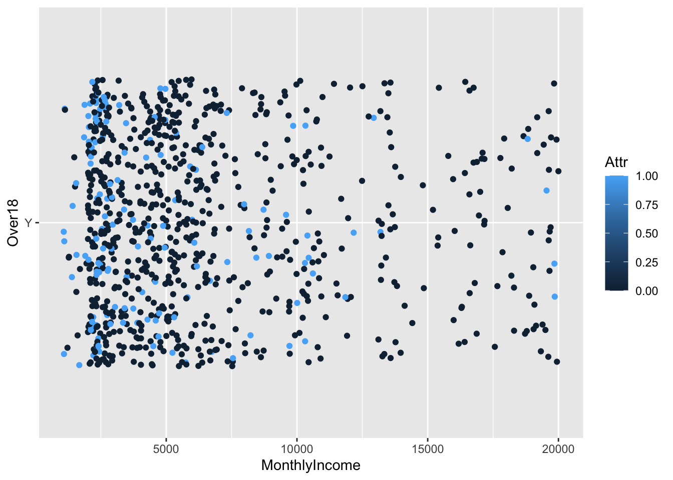
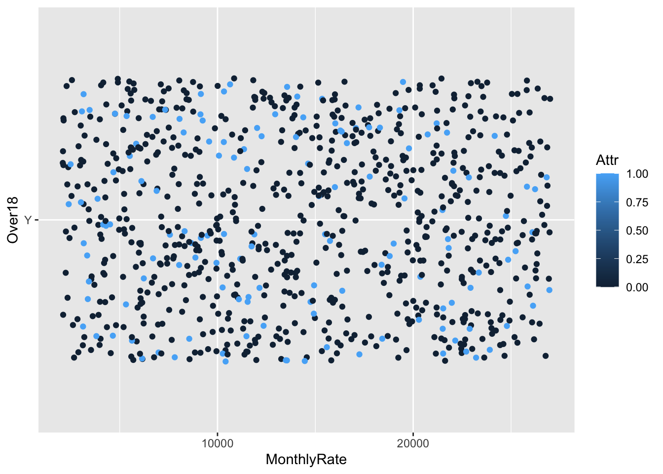
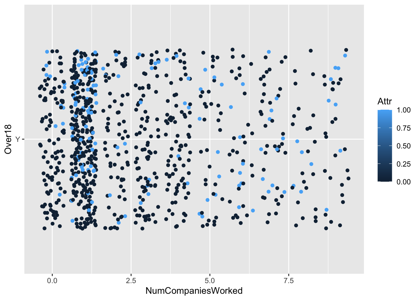
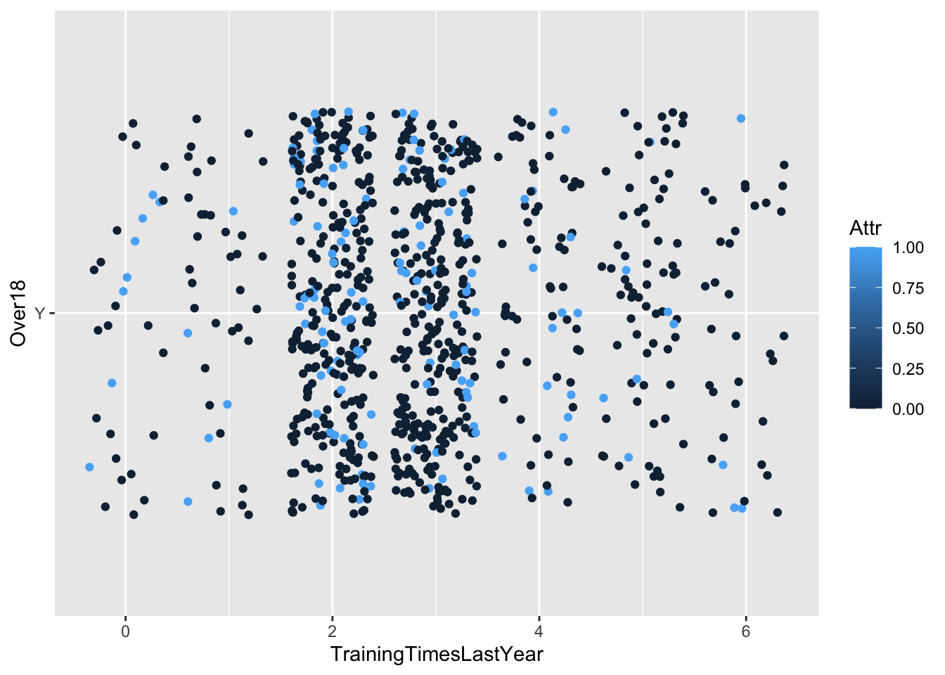
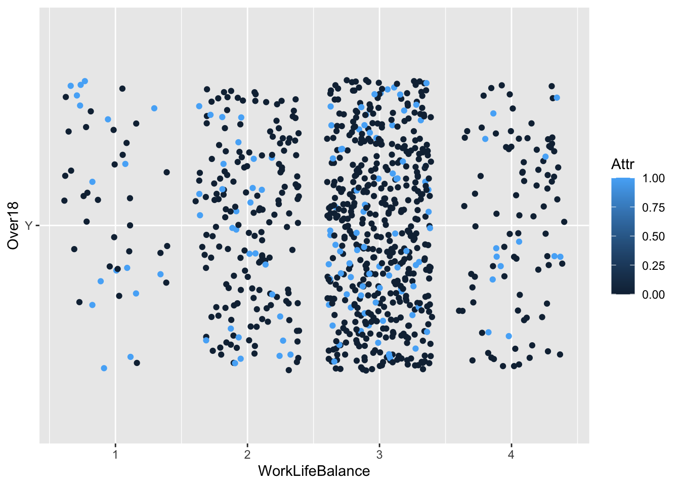
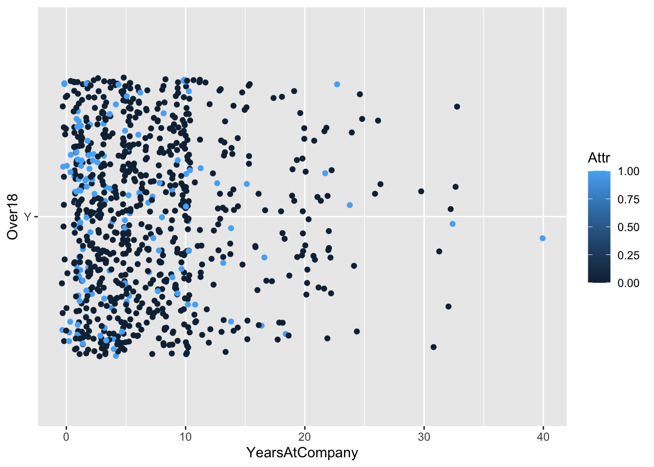
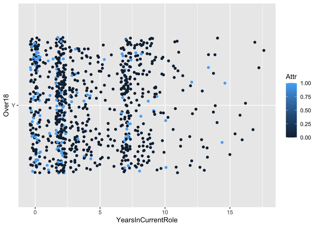
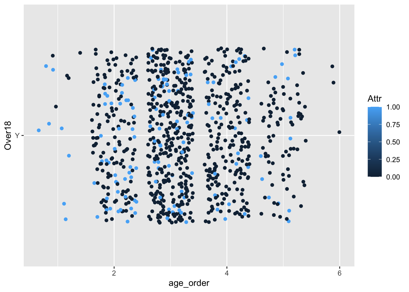
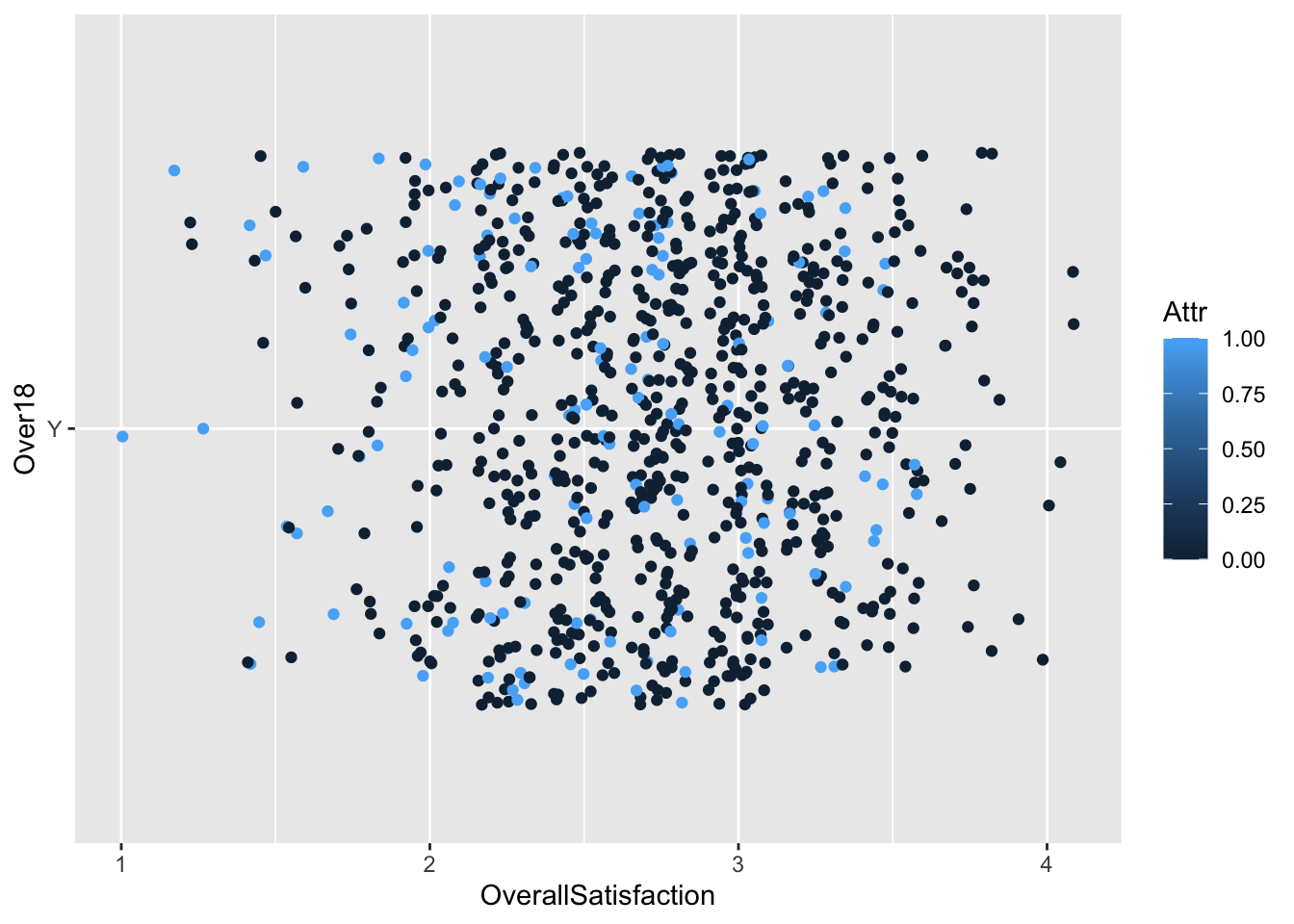
Investigate Key Categorization Attributes

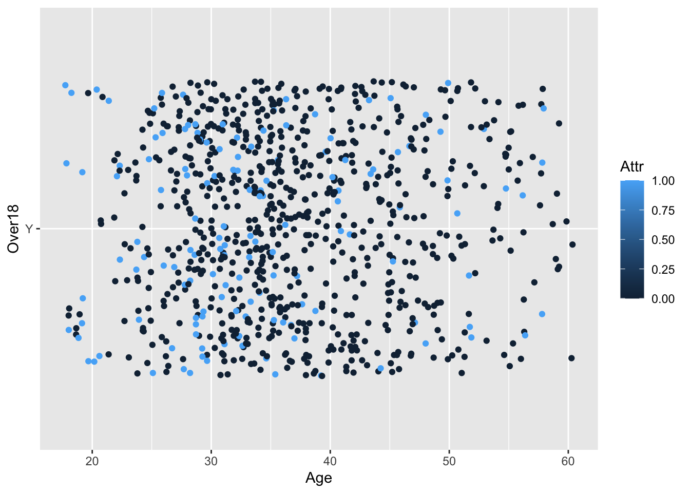
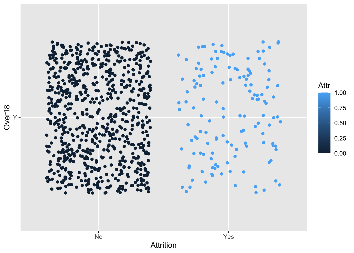
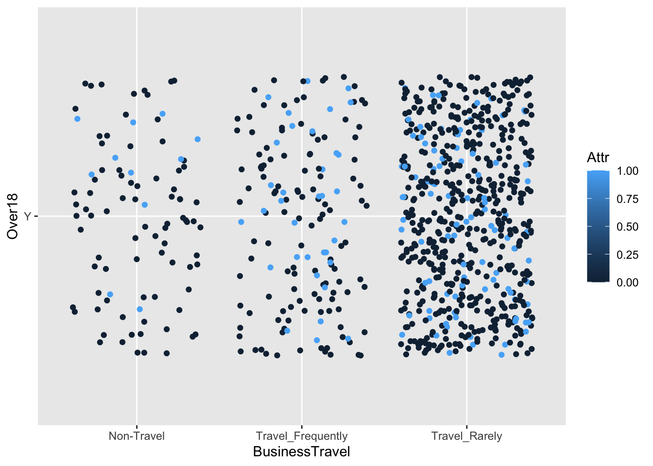
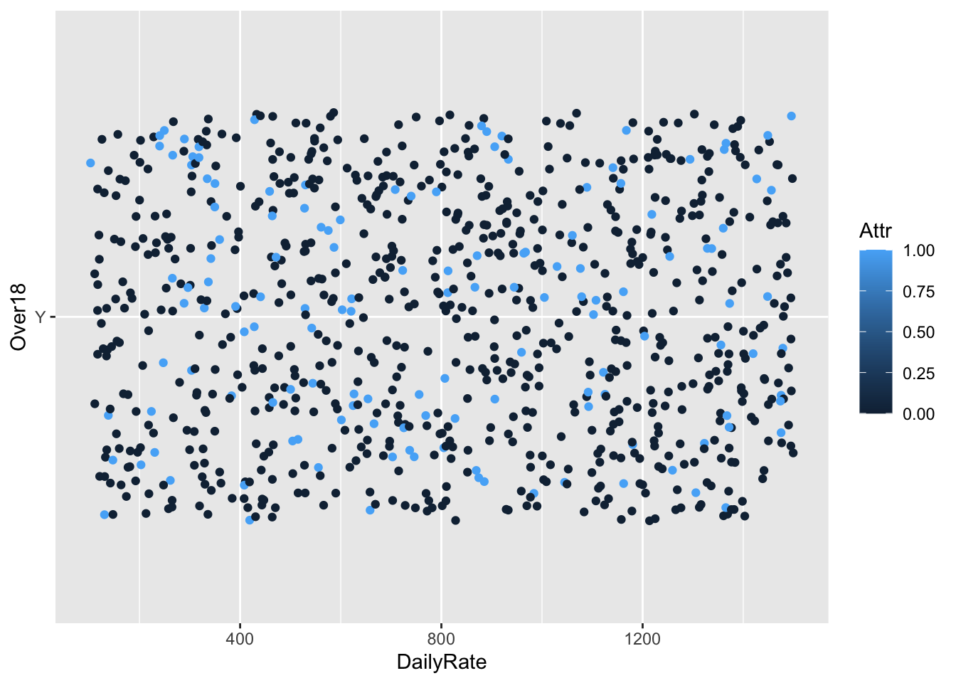
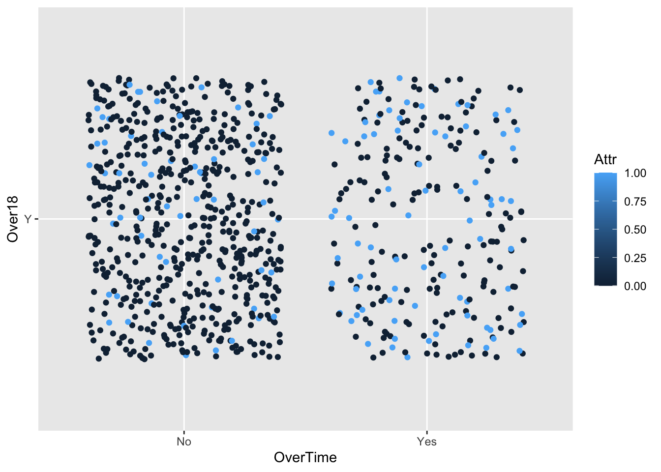
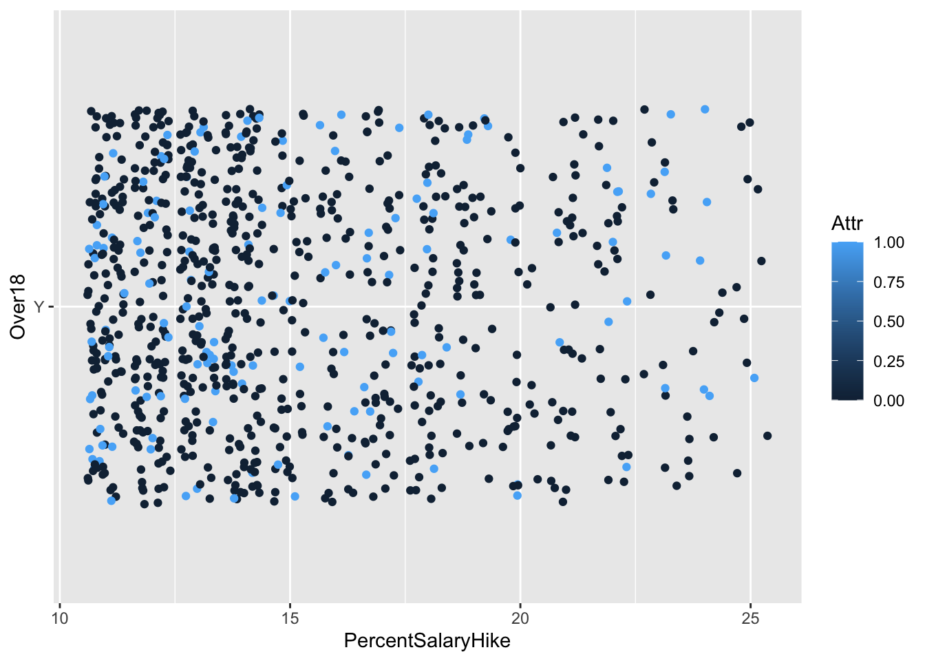
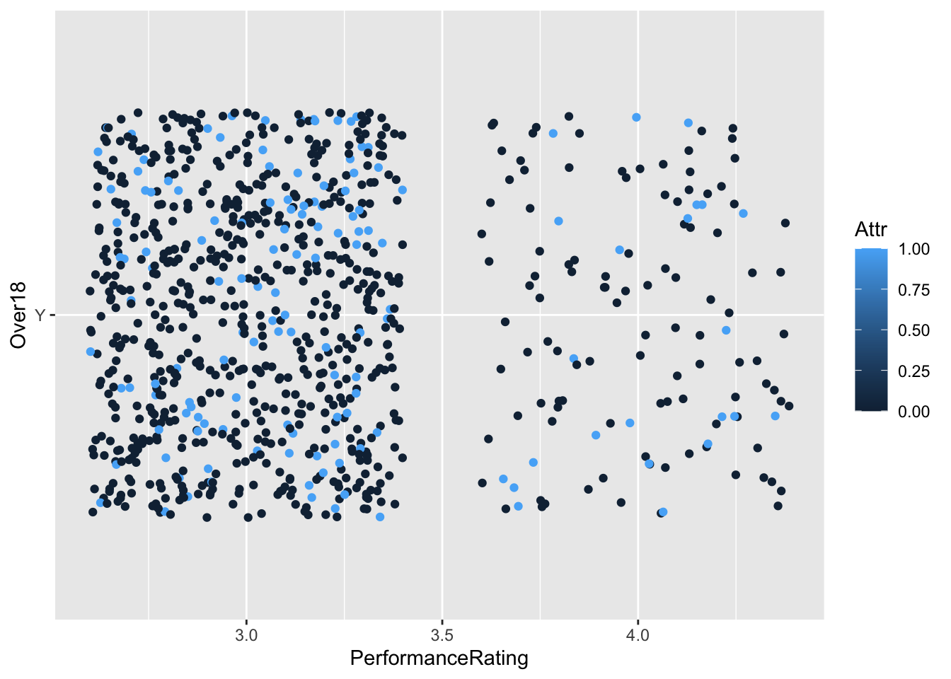
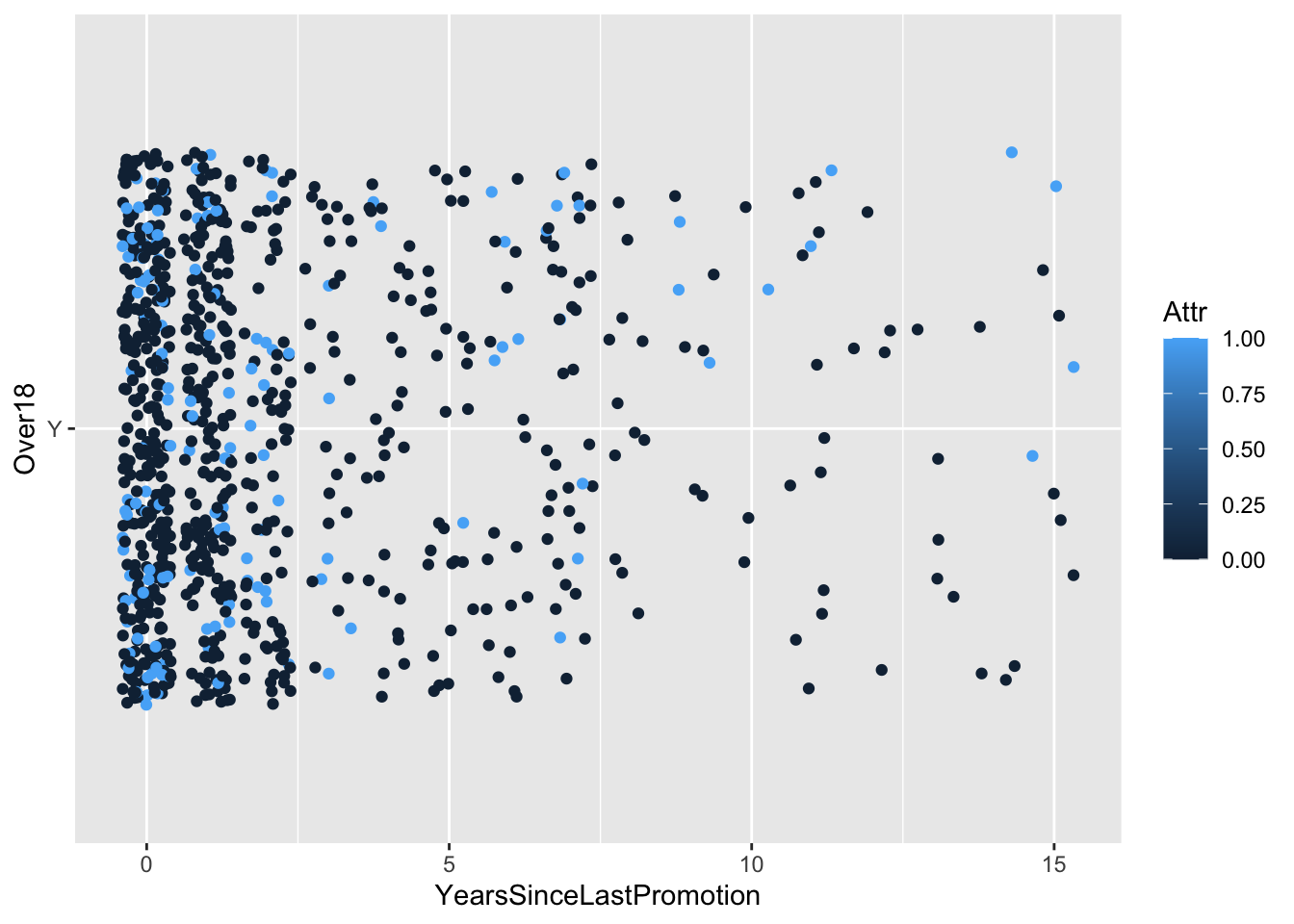
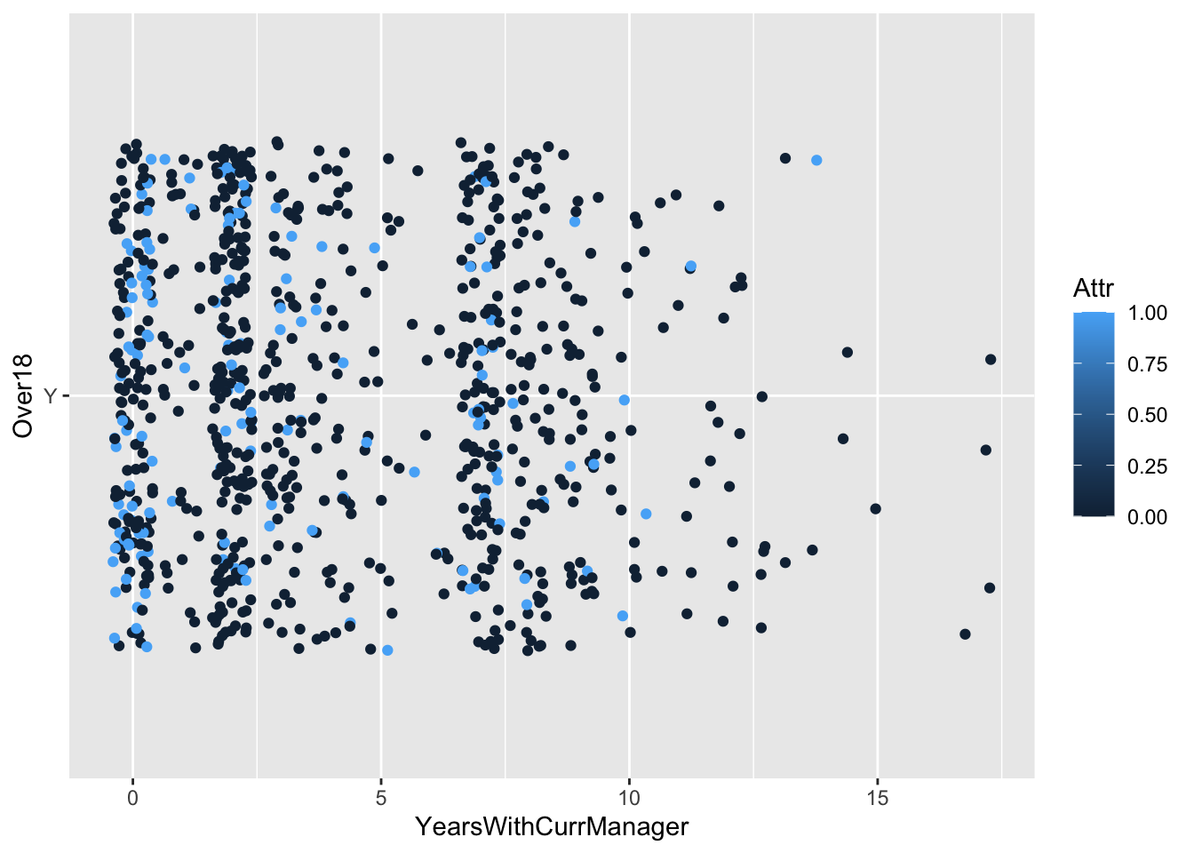
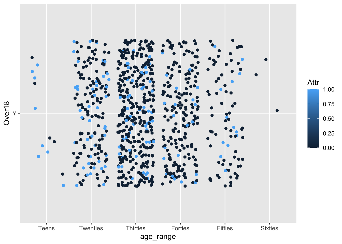
Use constant value Over18 for y value for consistent comparison

for(i in 2:40)
{

 p = ggplot(data = data, mapping = aes(x = data[,i], y = Over18, color = Attr)) + geom_point(position = "jitter") + xlab(colnames(data[i]))
 print(p)

}

Clean up data for modeling

data2 = select_if(data,is.numeric)
data2 = data2[,1:31]


data2_not = select(data,!is.numeric)
data2_not = data2_not[,2:9]

data2_not = data2_not %>% 
  mutate(BusinessTravelRank = case_when(
    grepl("Non-Travel", BusinessTravel) ~ 0,
    grepl("Travel_Rarely", BusinessTravel) ~ 1,
    grepl("Travel_Frequently", BusinessTravel) ~ 3
  )) %>%
  mutate(DepartmentRank = case_when(
    grepl("Research & Development", Department) ~ 1,
    grepl("Human Resources", Department) ~ 2,
    grepl("Sales", Department) ~ 3
  )) %>%
  mutate(EducationFieldRank = case_when(
    grepl("Life Sciences", EducationField) ~ 1,
    grepl("Medical", EducationField) ~ 2,
    grepl("Marketing", EducationField) ~ 3,
    grepl("Technical Degree", EducationField) ~ 4,
    grepl("Other", EducationField) ~ 5,
    grepl("Human Resources", EducationField) ~ 6
  )) %>%
  mutate(GenderRank = case_when(
    grepl("Male", Gender) ~ 0,
    grepl("Female", Gender) ~ 1
  )) %>%
  mutate(OvertimeRank = case_when(
    grepl("Yes", OverTime) ~ 0,
    grepl("No", OverTime) ~ 1
  ))

data2_not = select_if(data2_not,is.numeric)
  
data2 = cbind(data2,data2_not)

gg_miss_var(data2)

## Warning: It is deprecated to specify `guide = FALSE` to remove a guide. Please use `guide = "none"` instead.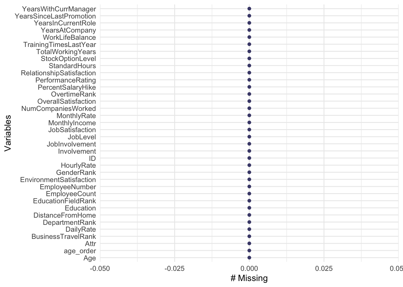

Classification: KNN

splitPerc = 0.75
trainInices = sample(1:dim(data2)[1], round(splitPerc * dim(data2)[1]))

train = data2[trainInices,]
test = data2[-trainInices,]


# Create model info dataframe
model_info = data.frame(matrix(ncol = 3, nrow = 100000))
colnames(model_info) = c("Model", "Sensitivity","Specificity")

tic = 1 # Ticker for loop

# Uncomment for k value loop
# for(l in 2:30)
#{
  for (i in 2:36)
  {
    for(j in i:36)
    {
      for(k in j:36)
      {
        classifications = knn(train[,c(i,j,k)], test[,c(i,j,k)], train$Attr, prob = TRUE, k = 11)
        table(classifications, test$Attr)
        x = confusionMatrix(table(classifications, test$Attr))
  
        # Comment for k valu eloop
        model_info$Model[tic]=(paste("Model for ",colnames(data2[i]), " and ", colnames(data2[j]), " and ", colnames(data2[k])))
  
        # Uncomment for k value loop
        # model_info$Model[tic]=(paste("Model for ",colnames(data2[i]), " and ", colnames(data2[j]), " and ", colnames(data2[k]), " and k = ", l))
  
        model_info$Sensitivity[tic] = x$byClass[1]
        model_info$Specificity[tic] = x$byClass[2]
  
        tic = tic + 1
      }
    }
  }
#} Uncomment for k value loop

output = model_info %>% 
  filter(!grepl("Attr",Model)) %>%
  arrange(-Specificity)

head(output)

##                                                                          Model Sensitivity Specificity
## 1     Model for  StockOptionLevel  and  OverallSatisfaction  and  OvertimeRank   0.9513514   0.3939394
## 2                   Model for  EmployeeCount  and  JobLevel  and  OvertimeRank   0.9243243   0.3636364
## 3 Model for  EnvironmentSatisfaction  and  StockOptionLevel  and  OvertimeRank   0.9567568   0.3636364
## 4                        Model for  JobLevel  and  JobLevel  and  OvertimeRank   0.9243243   0.3636364
## 5               Model for  JobLevel  and  PerformanceRating  and  OvertimeRank   0.9243243   0.3636364
## 6                   Model for  JobLevel  and  StandardHours  and  OvertimeRank   0.9243243   0.3636364

Classification: Naive Bayes

bayes_model = naiveBayes(Attr~., data = data2)
predict(bayes_model, data2)

##   [1] 0 0 0 0 1 0 0 0 0 0 0 0 0 1 0 0 0 0 0 0 0 0 0 0 0 0 0 1 1 0 0 0 0 0 0 1 0 0 0 0 0 0 0 0 0 0 1 0 1 1 0 0 0 0 0 0 0 0 0 1 0 0 0 1 1 0
##  [67] 0 0 0 0 0 0 1 0 0 0 0 0 0 0 1 0 0 0 0 0 0 1 0 0 0 0 1 0 0 0 0 0 0 0 0 0 0 1 0 0 0 0 0 0 1 0 0 0 0 0 0 1 0 0 0 1 0 0 0 0 1 0 0 0 1 0
## [133] 0 0 0 0 1 0 1 0 0 0 0 0 0 0 0 0 1 1 1 0 0 0 0 1 0 0 0 0 0 0 0 0 0 1 0 0 0 0 0 0 0 0 0 1 0 1 0 0 0 0 0 0 0 0 0 0 0 0 0 0 0 0 1 0 0 0
## [199] 0 1 0 0 0 1 0 1 1 1 0 0 0 0 0 0 1 0 0 0 0 1 0 0 0 1 0 0 0 1 1 0 0 0 0 0 0 0 0 0 1 0 0 0 0 1 0 0 0 0 0 0 0 0 0 0 0 0 0 0 0 1 1 1 0 0
## [265] 0 0 0 0 0 0 0 0 0 0 0 0 1 0 1 0 0 0 0 0 0 0 1 0 0 0 0 0 0 0 0 0 0 1 1 1 0 0 0 0 0 1 0 0 0 0 0 0 0 0 1 0 0 1 0 1 0 0 0 0 0 0 0 0 0 0
## [331] 0 0 0 0 0 0 0 0 0 0 1 1 0 0 0 0 0 0 1 0 0 0 1 0 0 0 1 1 0 0 0 1 0 0 0 0 0 0 0 0 0 0 0 0 1 0 0 0 1 1 0 0 0 1 0 0 0 0 0 1 0 1 0 0 0 1
## [397] 0 1 0 0 0 0 0 0 1 0 0 0 0 0 1 0 1 0 1 0 0 0 0 0 0 0 1 0 1 0 0 1 1 0 1 0 1 1 0 0 0 0 1 0 0 0 1 0 0 0 0 0 0 0 0 0 0 0 0 0 0 1 0 0 0 0
## [463] 0 0 1 0 0 0 1 0 0 1 0 0 0 0 0 1 1 0 0 0 0 0 0 1 0 0 1 0 0 0 1 0 0 0 0 0 0 1 0 1 0 0 0 0 1 0 0 0 0 0 0 0 1 0 1 0 0 0 0 1 0 0 0 0 0 1
## [529] 0 0 0 0 0 0 1 0 0 0 1 0 0 0 1 0 0 0 0 0 0 0 0 0 1 0 0 0 0 0 0 0 0 0 1 0 0 0 0 0 0 0 0 1 0 0 0 0 1 0 0 0 0 0 1 1 0 0 0 1 0 0 1 1 1 0
## [595] 0 0 0 0 1 1 1 0 0 0 1 0 0 0 0 1 0 0 0 1 0 0 0 1 0 0 1 0 0 0 1 0 0 0 0 0 0 0 0 0 0 0 0 0 0 0 0 0 0 1 1 0 1 1 0 1 0 0 0 0 1 1 0 0 0 0
## [661] 0 0 0 0 0 0 0 1 0 0 0 0 0 1 1 0 0 0 0 0 1 0 0 0 1 0 0 0 1 0 0 0 0 1 0 1 0 0 1 0 1 0 0 1 0 0 0 0 0 0 0 0 0 0 0 1 0 0 0 0 0 0 0 0 0 0
## [727] 0 0 1 0 0 1 1 0 0 0 0 0 0 1 1 0 0 1 1 1 1 0 1 0 1 1 0 0 0 1 0 0 0 0 1 0 0 0 1 1 0 1 0 0 0 0 0 1 0 0 0 0 0 0 1 0 0 0 0 0 0 0 0 0 0 0
## [793] 0 0 0 1 0 1 1 0 0 0 0 0 0 0 1 0 0 1 0 1 1 0 0 0 1 0 0 1 0 0 0 0 0 0 0 1 0 0 0 1 0 1 0 0 0 0 0 0 1 0 0 0 1 0 1 0 0 0 1 0 0 0 1 0 0 0
## [859] 0 0 0 0 1 0 0 0 0 0 0 0
## Levels: 0 1

confusionMatrix(table(predict(bayes_model,data2), data2$Attr))

## Confusion Matrix and Statistics
## 
##    
##       0   1
##   0 639  53
##   1  91  87
##                                           
##                Accuracy : 0.8345          
##                  95% CI : (0.8081, 0.8586)
##     No Information Rate : 0.8391          
##     P-Value [Acc > NIR] : 0.664134        
##                                           
##                   Kappa : 0.4477          
##                                           
##  Mcnemar's Test P-Value : 0.002047        
##                                           
##             Sensitivity : 0.8753          
##             Specificity : 0.6214          
##          Pos Pred Value : 0.9234          
##          Neg Pred Value : 0.4888          
##              Prevalence : 0.8391          
##          Detection Rate : 0.7345          
##    Detection Prevalence : 0.7954          
##       Balanced Accuracy : 0.7484          
##                                           
##        'Positive' Class : 0               
##

# Note - while we initially worked to construct a knn model, the max specificity we could obtain was roughly 30%. Since this was below our 60% threshold, we moved forward with a probability based naive bayes model instead.

Linear Regression Model Investigation for correlation

for(i in 2:36)
{

 p = ggplot(data = data2, mapping = aes(x = data2[,i], y = MonthlyIncome,)) + geom_point(position = "jitter") + geom_smooth(method = "lm") + xlab(colnames(data2[i]))
 print(p)

}

## `geom_smooth()` using formula 'y ~ x'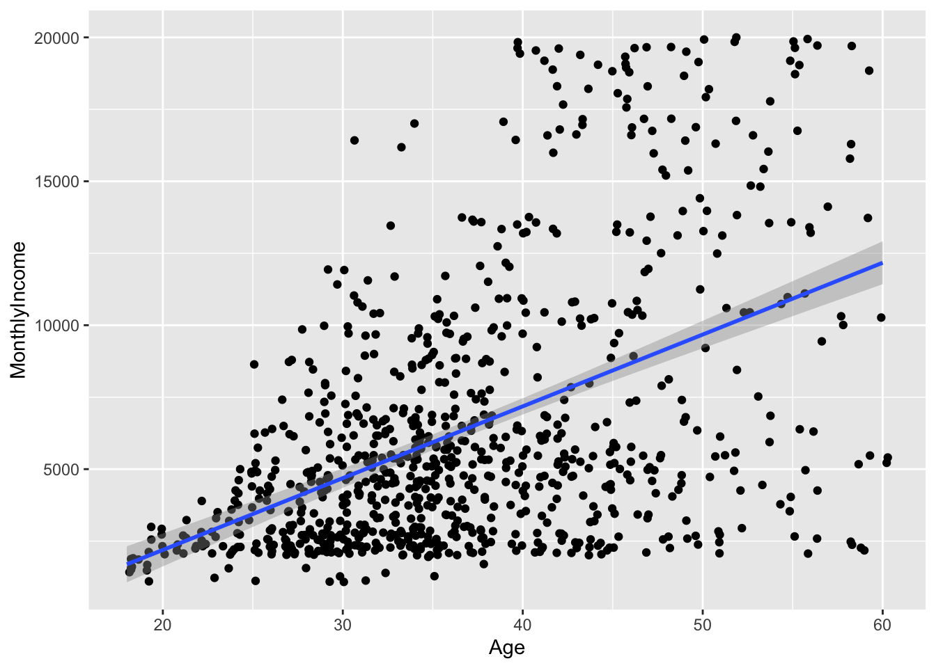

## `geom_smooth()` using formula 'y ~ x'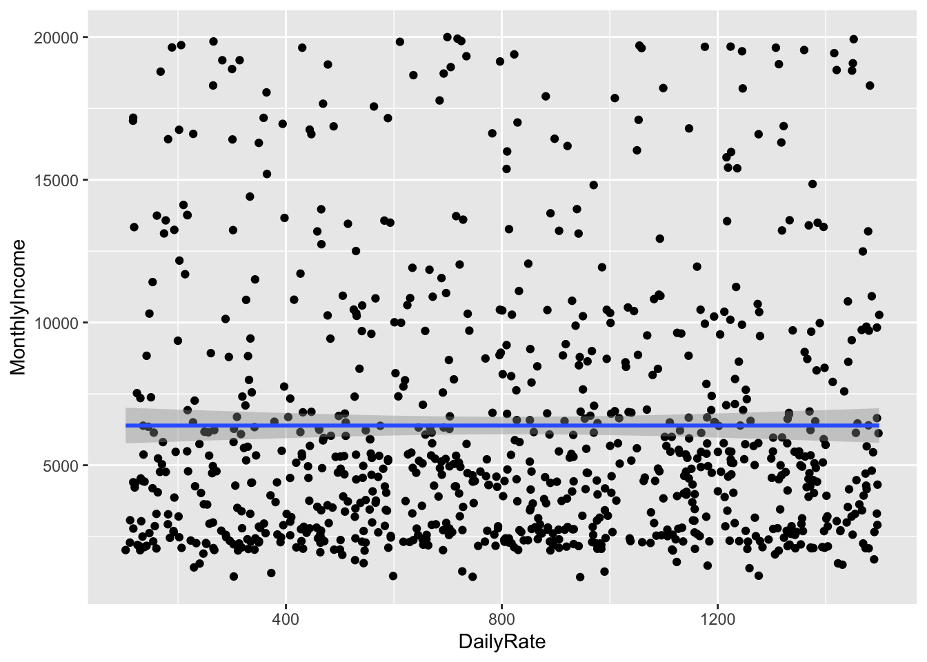

## `geom_smooth()` using formula 'y ~ x'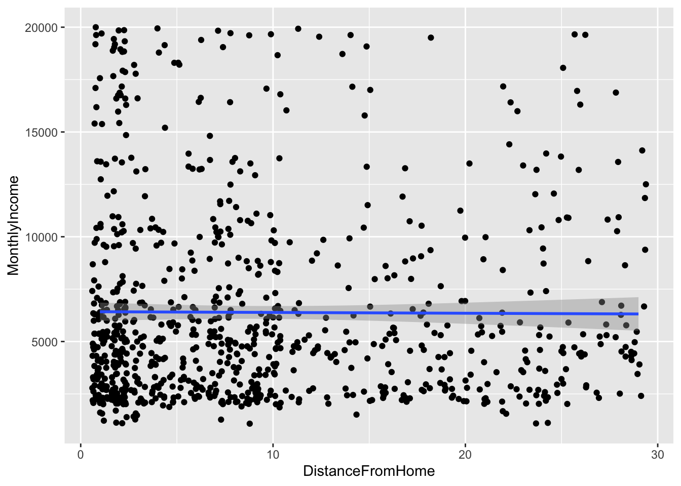

## `geom_smooth()` using formula 'y ~ x'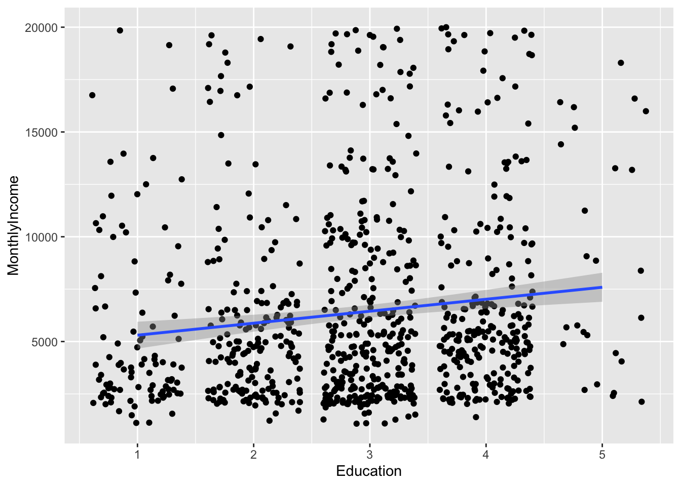

## `geom_smooth()` using formula 'y ~ x'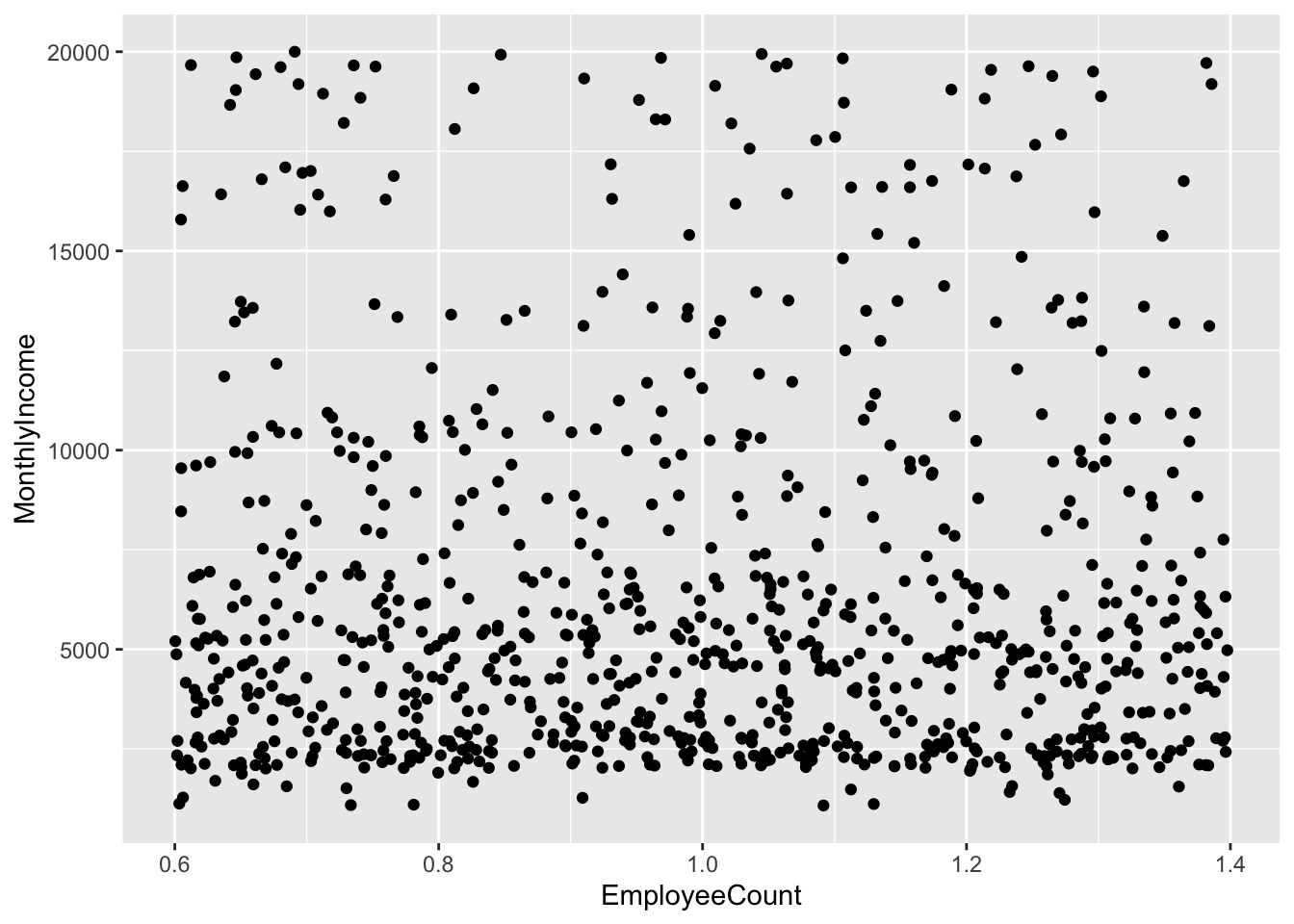

## `geom_smooth()` using formula 'y ~ x'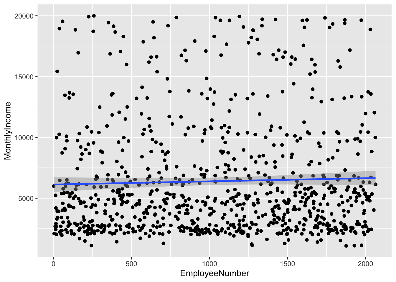

## `geom_smooth()` using formula 'y ~ x'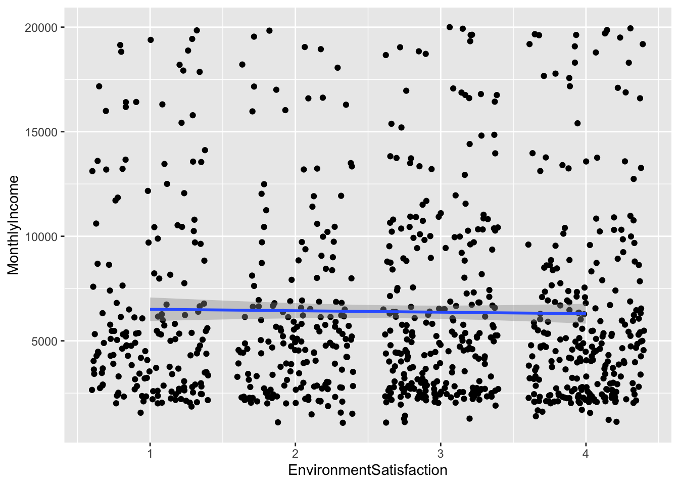

## `geom_smooth()` using formula 'y ~ x'

## `geom_smooth()` using formula 'y ~ x'

## `geom_smooth()` using formula 'y ~ x'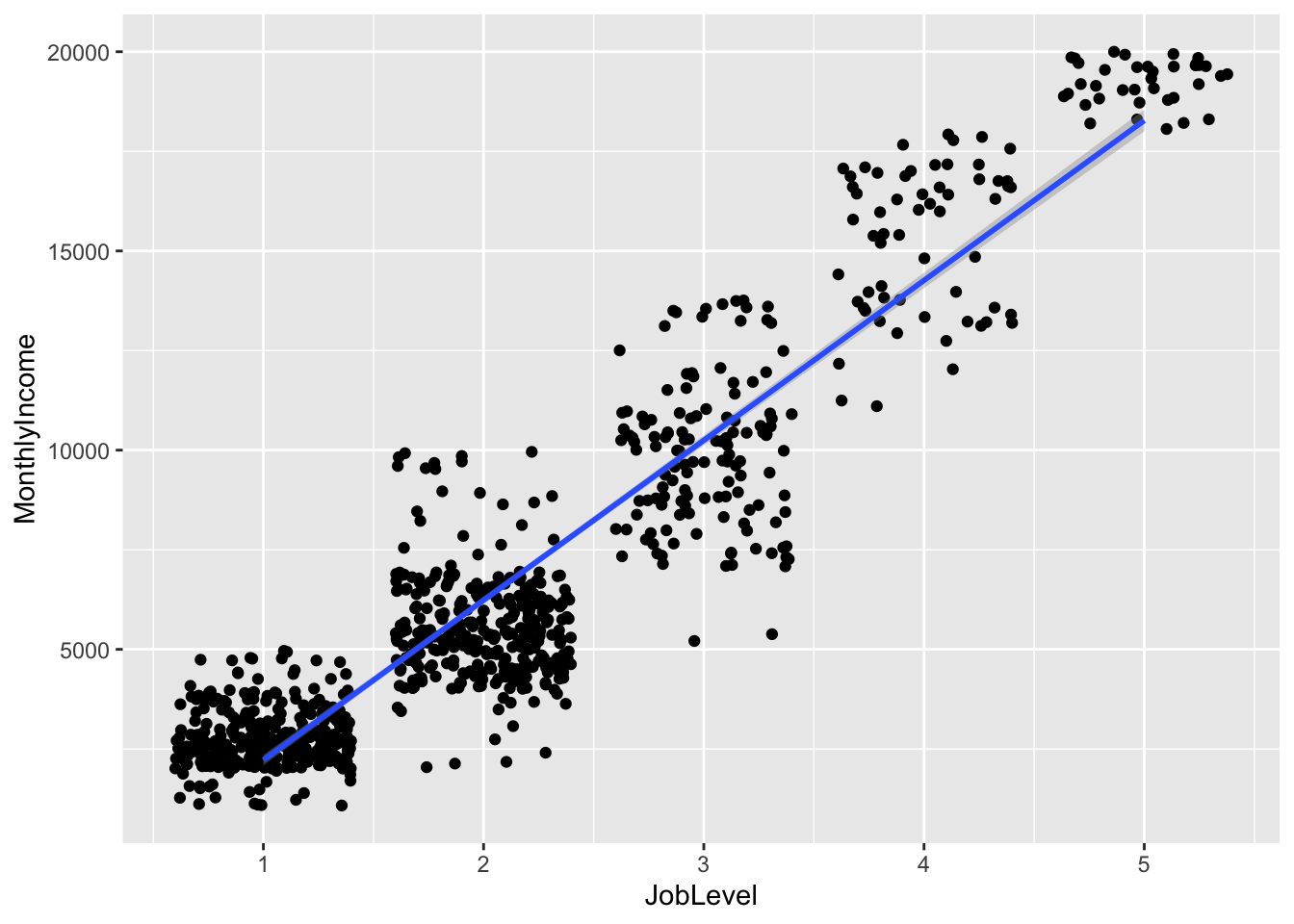

## `geom_smooth()` using formula 'y ~ x'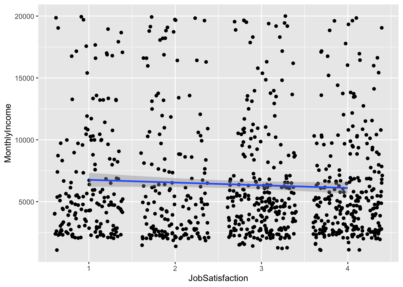

## `geom_smooth()` using formula 'y ~ x'

## `geom_smooth()` using formula 'y ~ x'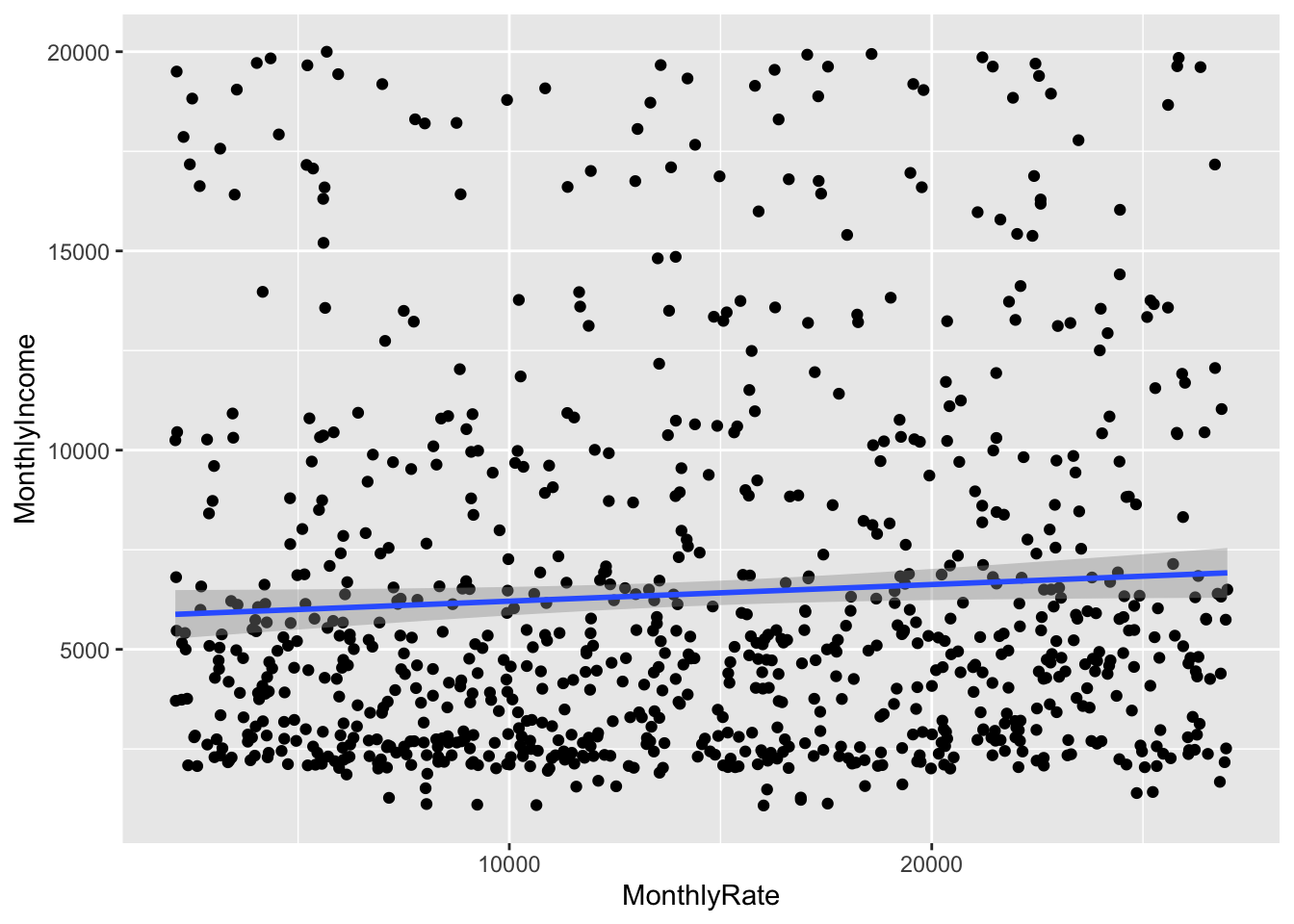

## `geom_smooth()` using formula 'y ~ x'

## `geom_smooth()` using formula 'y ~ x'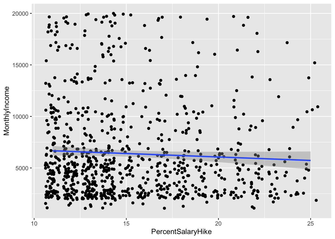

## `geom_smooth()` using formula 'y ~ x'

## `geom_smooth()` using formula 'y ~ x'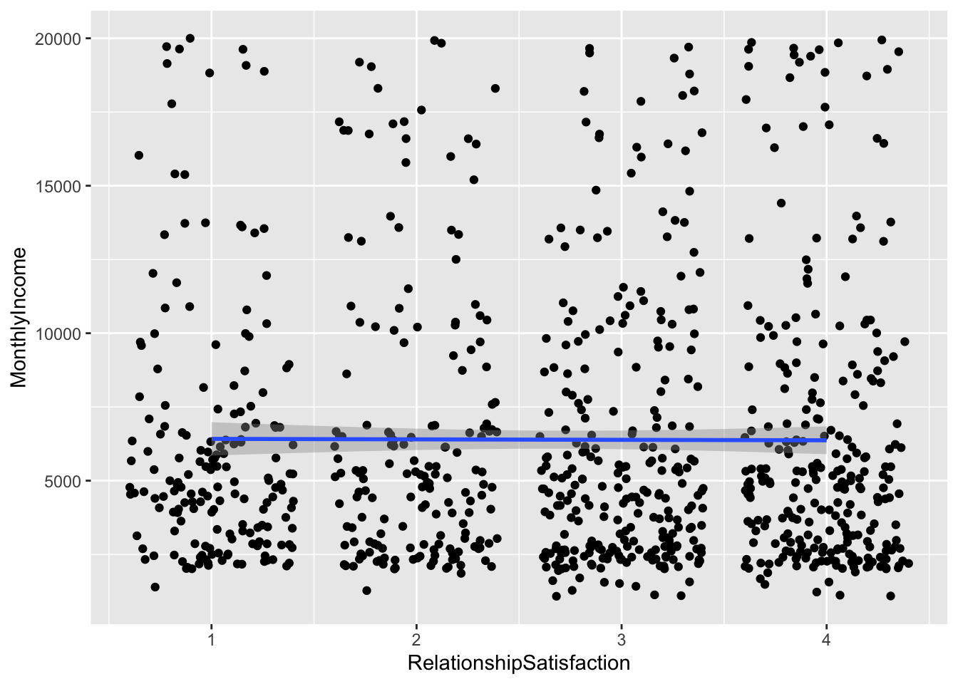

## `geom_smooth()` using formula 'y ~ x'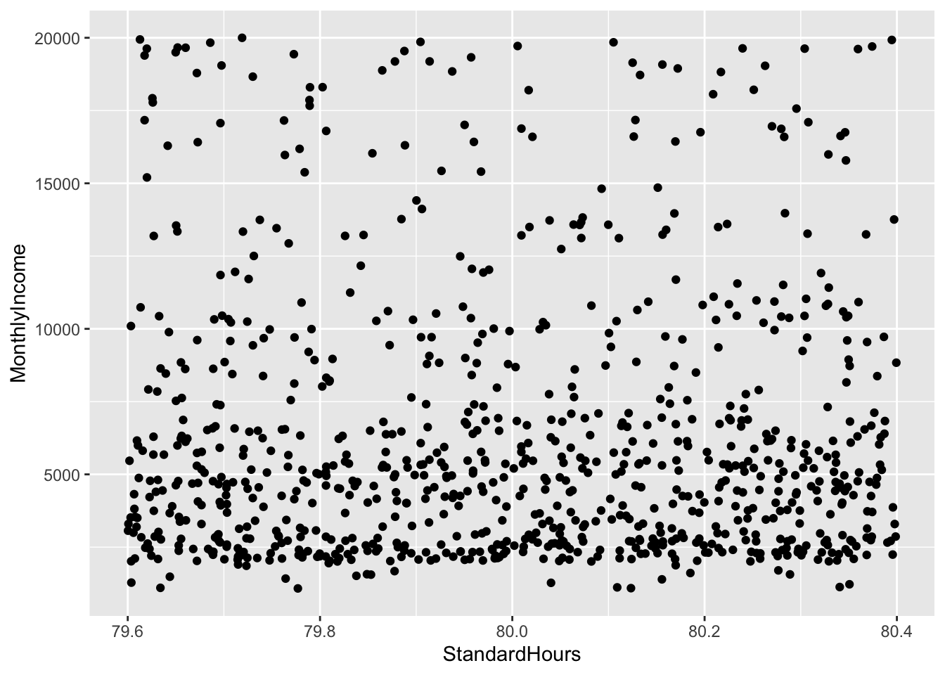

## `geom_smooth()` using formula 'y ~ x'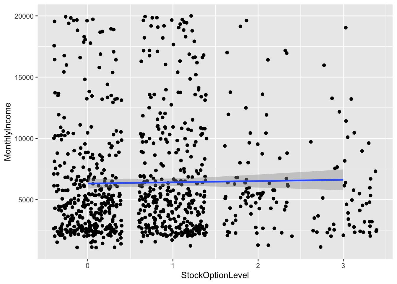

## `geom_smooth()` using formula 'y ~ x'

## `geom_smooth()` using formula 'y ~ x'

## `geom_smooth()` using formula 'y ~ x'

## `geom_smooth()` using formula 'y ~ x'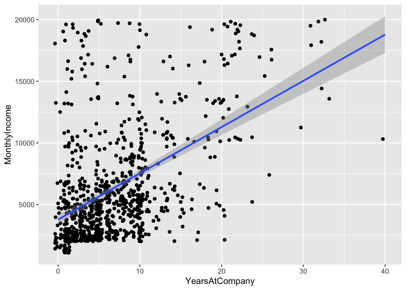

## `geom_smooth()` using formula 'y ~ x'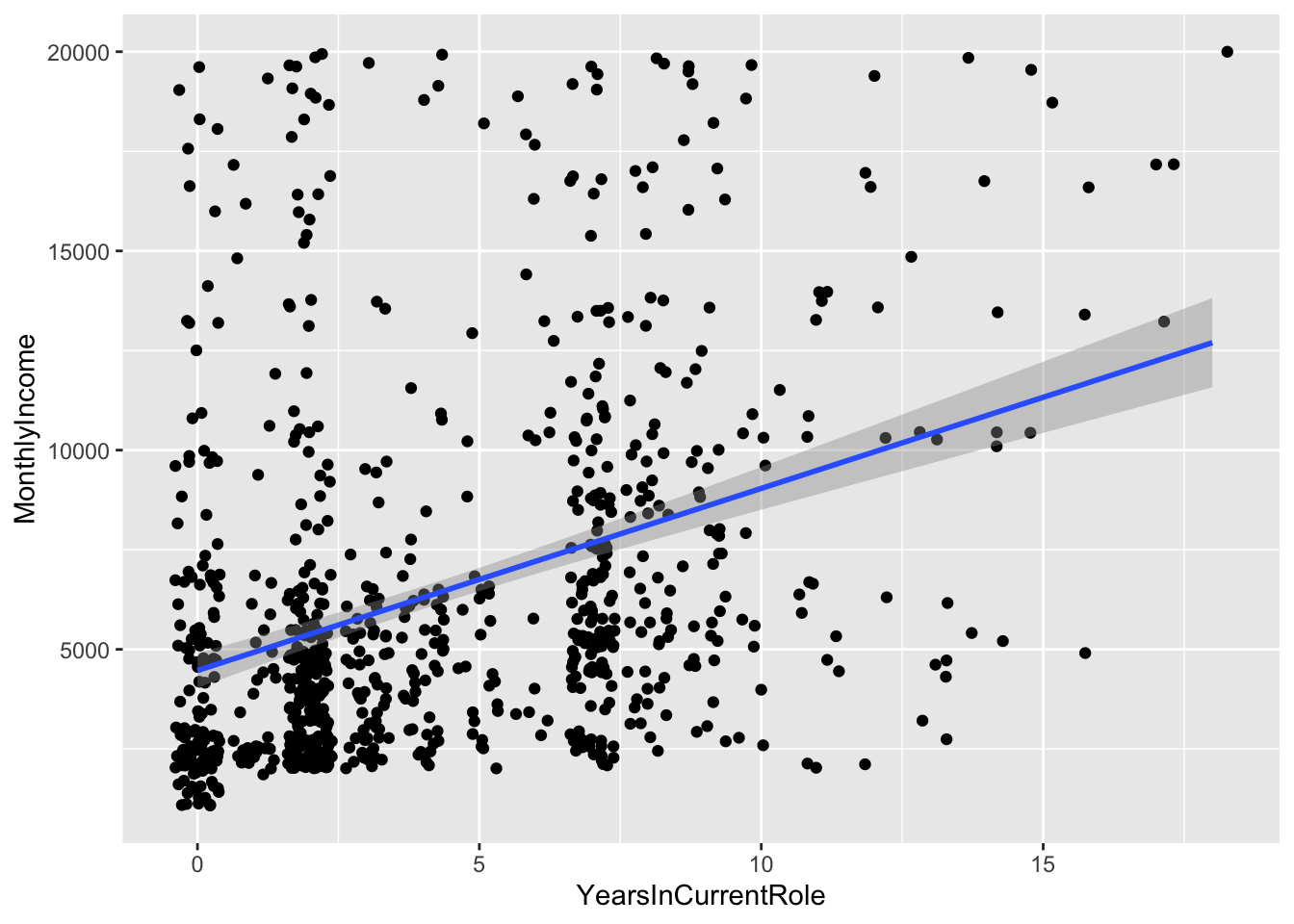

## `geom_smooth()` using formula 'y ~ x'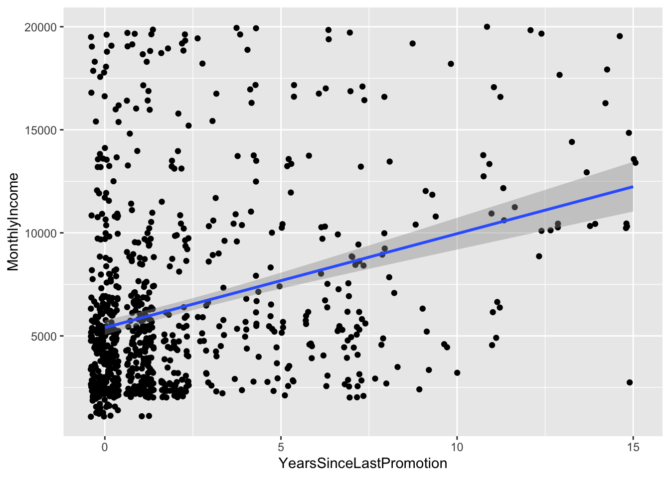

## `geom_smooth()` using formula 'y ~ x'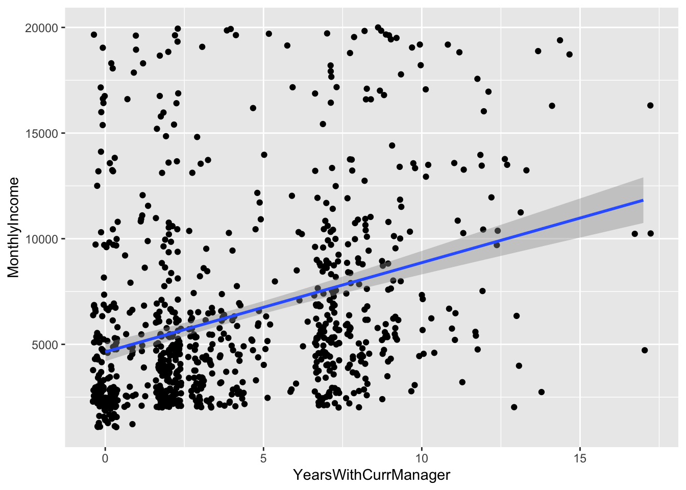

## `geom_smooth()` using formula 'y ~ x'

## `geom_smooth()` using formula 'y ~ x'

## `geom_smooth()` using formula 'y ~ x'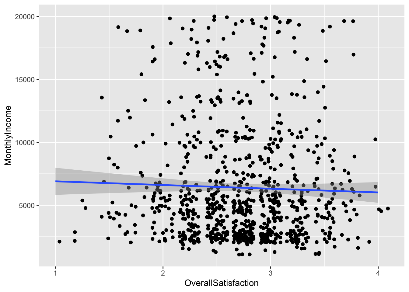

## `geom_smooth()` using formula 'y ~ x'

## `geom_smooth()` using formula 'y ~ x'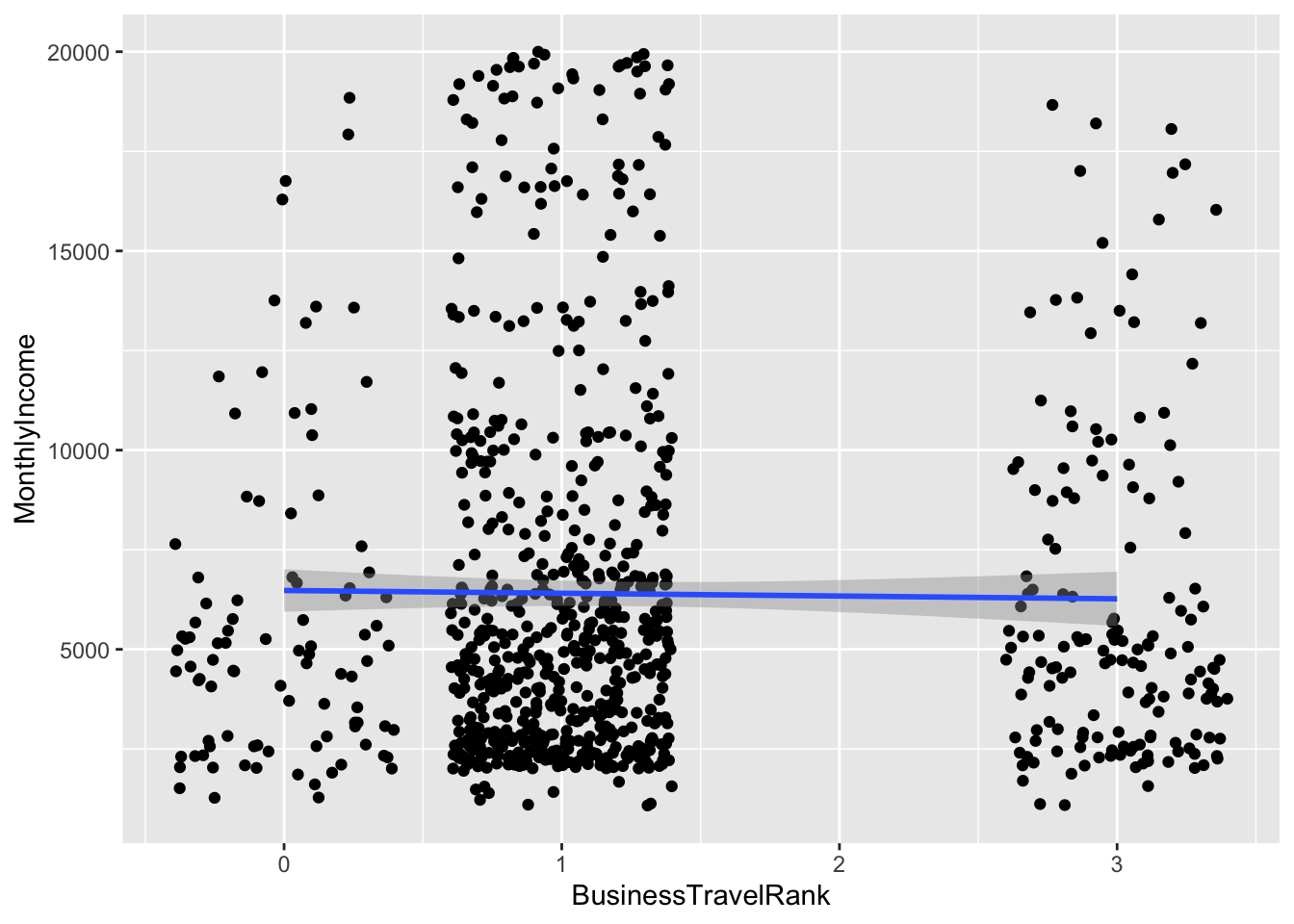

## `geom_smooth()` using formula 'y ~ x'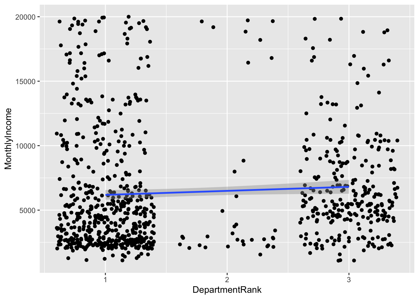

## `geom_smooth()` using formula 'y ~ x'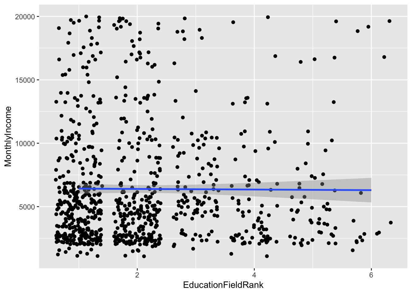

## `geom_smooth()` using formula 'y ~ x'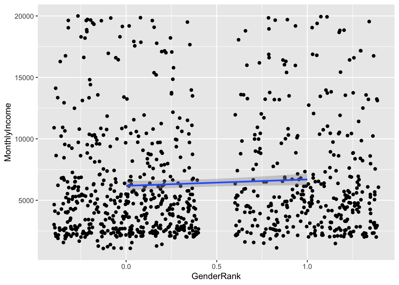

## `geom_smooth()` using formula 'y ~ x'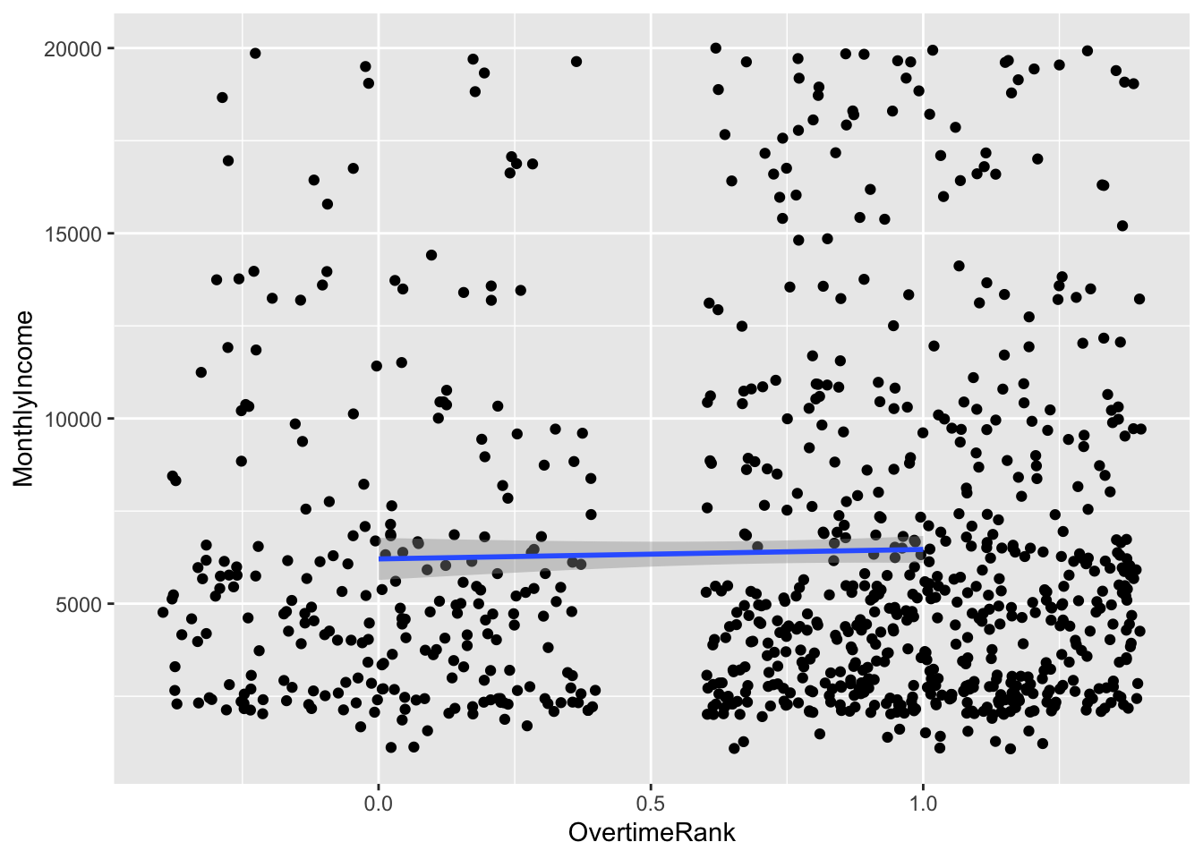

Top Attributes:

Age
Education
Job Level
Total Working Years
Years at Company
Years in current role
Years since last promotion
Years with current manager

Collinearity

Job Level Total Working Years, Years at Company, Years in Current Role, Years since Last promotion, and Years with current manager are all likely correlated, so we will use the one with the strongest correlation with income: Job Level

Linear Regression Model with Top 3 correlating attributes

fit = lm(MonthlyIncome ~ Age + JobLevel + Education , data = data2) 
summary(fit)

## 
## Call:
## lm(formula = MonthlyIncome ~ Age + JobLevel + Education, data = data2)
## 
## Residuals:
##     Min      1Q  Median      3Q     Max 
## -5121.1  -950.7    68.5   740.9  3852.0 
## 
## Coefficients:
##              Estimate Std. Error t value Pr(>|t|)    
## (Intercept) -2310.409    223.920 -10.318  < 2e-16 ***
## Age            19.041      6.193   3.075  0.00217 ** 
## JobLevel     3940.417     49.922  78.932  < 2e-16 ***
## Education     -12.211     47.825  -0.255  0.79854    
## ---
## Signif. codes:  0 '***' 0.001 '**' 0.01 '*' 0.05 '.' 0.1 ' ' 1
## 
## Residual standard error: 1407 on 866 degrees of freedom
## Multiple R-squared:  0.9066, Adjusted R-squared:  0.9063 
## F-statistic:  2804 on 3 and 866 DF,  p-value: < 2.2e-16

RSS = c(crossprod(fit$residuals))
MSE = RSS/length(fit$residuals)
RMSE = sqrt(MSE)
print(RMSE)

## [1] 1403.957

Testing other regression combinations

model_df = data.frame(matrix(ncol = 6, nrow = 100000))
colnames(model_df) = c("Model", "Intercept","First", "Second", "Third", "RMSE")

tic = 0
  for (i in 2:36) 
  {
    for(j in i:36)
    {
      for(k in j:36)
      {
        
        fit = lm(MonthlyIncome ~ data2[,i] + data2[,j] + data2[,k] , data = data2) 
        x = summary(fit)
        RSS = c(crossprod(fit$residuals))
        MSE = RSS/length(fit$residuals)
        RMSE = sqrt(MSE)
        
        model_df$Model[tic] = paste(colnames(data2[i]), " and ", colnames(data2[j]), " and ", colnames(data2[k]))
        model_df$Intercept[tic] = x$coefficients[13]
        model_df$First[tic] = x$coefficients[14]
        model_df$Second[tic] = x$coefficients[15]
        model_df$Third[tic] = x$coefficients[16]
        model_df$RMSE[tic] = RMSE
        
        tic = tic + 1
      }
    }
  }

output = model_df %>%
  filter(!grepl("MonthlyIncome", Model)) %>%
  filter(!is.na(Intercept)) %>%
  arrange(RMSE)

head(output)

##                                                            Model    Intercept         First        Second        Third     RMSE
## 1    JobLevel  and  TotalWorkingYears  and  YearsWithCurrManager 3.875726e-54 2.198417e-280  1.014850e-10 6.182710e-05 1374.498
## 2          JobLevel  and  TotalWorkingYears  and  DepartmentRank 8.112807e-31 5.599165e-278  1.695192e-06 1.011159e-04 1375.237
## 3          JobLevel  and  TotalWorkingYears  and  YearsAtCompany 1.028183e-59 1.245489e-279  2.636976e-10 1.578655e-03 1379.319
## 4      JobLevel  and  TotalWorkingYears  and  YearsInCurrentRole 6.344685e-56 2.816539e-279  6.816520e-10 2.514322e-03 1380.000
## 5        DistanceFromHome  and  JobLevel  and  TotalWorkingYears 2.183966e-44  1.055329e-02 7.578019e-279 4.793820e-08 1382.068
## 6 JobLevel  and  TotalWorkingYears  and  YearsSinceLastPromotion 1.781831e-61 1.595467e-277  9.082826e-09 8.836960e-02 1384.973

Findings: JobLevel, age_order and DepartmentRank yield the lowest RMSE from the attribute set combinataions that are not collinear

Final Linear Regression Model

lin_fit = lm(MonthlyIncome ~ JobLevel + age_order + DepartmentRank , data = data2) 
summary(lin_fit)

## 
## Call:
## lm(formula = MonthlyIncome ~ JobLevel + age_order + DepartmentRank, 
##     data = data2)
## 
## Residuals:
##     Min      1Q  Median      3Q     Max 
## -5279.4  -900.4    28.7   823.6  4131.7 
## 
## Coefficients:
##                Estimate Std. Error t value Pr(>|t|)    
## (Intercept)    -1855.89     191.46  -9.693  < 2e-16 ***
## JobLevel        3971.23      49.20  80.720  < 2e-16 ***
## age_order        165.89      56.79   2.921  0.00358 ** 
## DepartmentRank  -232.00      51.71  -4.486 8.23e-06 ***
## ---
## Signif. codes:  0 '***' 0.001 '**' 0.01 '*' 0.05 '.' 0.1 ' ' 1
## 
## Residual standard error: 1390 on 866 degrees of freedom
## Multiple R-squared:  0.9089, Adjusted R-squared:  0.9086 
## F-statistic:  2881 on 3 and 866 DF,  p-value: < 2.2e-16

RSS = c(crossprod(lin_fit$residuals))
MSE = RSS/length(lin_fit$residuals)
RMSE = sqrt(MSE)
print(RMSE)

## [1] 1386.747

Top Three Factors for Attrition

Age
Involvement
Satisfaction Score

Age vs % Attrition

data %>%
  group_by(age_range) %>%
  summarize(attrition_count = sum(Attr), Count = n(), perc_attrition = sum(Attr)/n())  %>%
  ggplot(aes(x = age_range, y = perc_attrition, fill = age_range)) +
  geom_bar(stat = "identity") +
  ggtitle("% Attrition by Age") +
  xlab("Age") +
  ylab("% Attrition") +
  theme(legend.position = "none")

data %>%
  group_by(age_range, age_order) %>%
  summarize(attrition_count = sum(Attr), Count = n(), perc_attrition = sum(Attr)/n())  %>%
  ggplot(aes(x = age_order, y = perc_attrition)) +
  geom_point() +
  geom_smooth(method = "lm") +
  ggtitle("% Attrition by Age") +
  xlab("Age Rank") +
  ylab("% Attrition") +
  theme(legend.position = "none")

## `summarise()` has grouped output by 'age_range'. You can override using the `.groups` argument.

## `geom_smooth()` using formula 'y ~ x'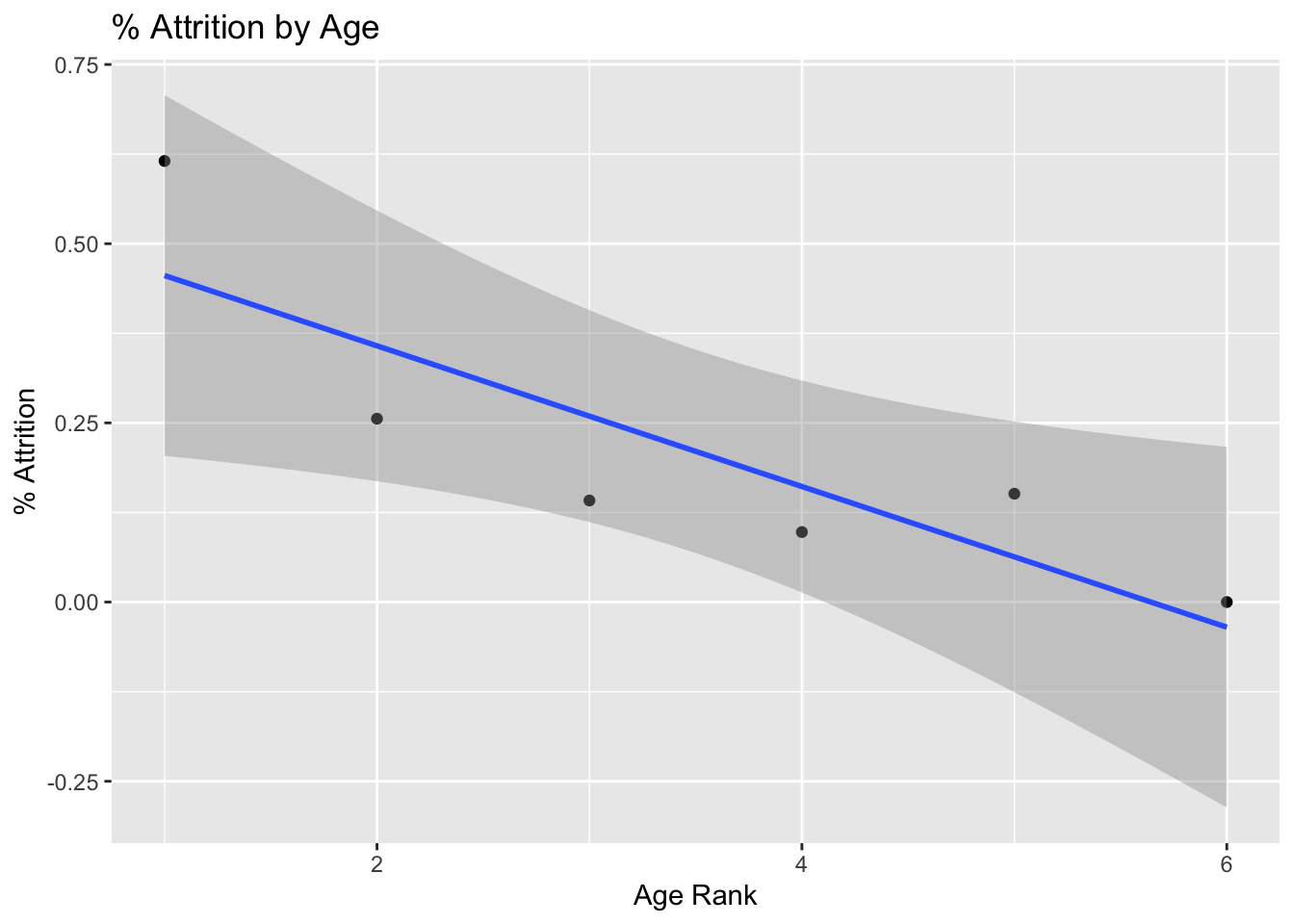

Satisfaction Score vs % Attrition

data = data %>%
  mutate(OverallSatisfaction = (JobSatisfaction+EnvironmentSatisfaction+WorkLifeBalance+RelationshipSatisfaction)/4)

data %>%
  group_by(OverallSatisfaction) %>%
   summarize(perc_attrition = sum(Attr)/n()) %>%
  ggplot(aes(x = OverallSatisfaction, perc_attrition)) +
  geom_point() +
  geom_smooth(method = "lm") +
  ylim(0,1) + 
  ggtitle("% Attrition by Satisfaction Score") +
  xlab("Score") +
  ylab("% Attrition") +
  theme(legend.position = "none")

## `geom_smooth()` using formula 'y ~ x'

## Warning: Removed 10 rows containing missing values (geom_smooth).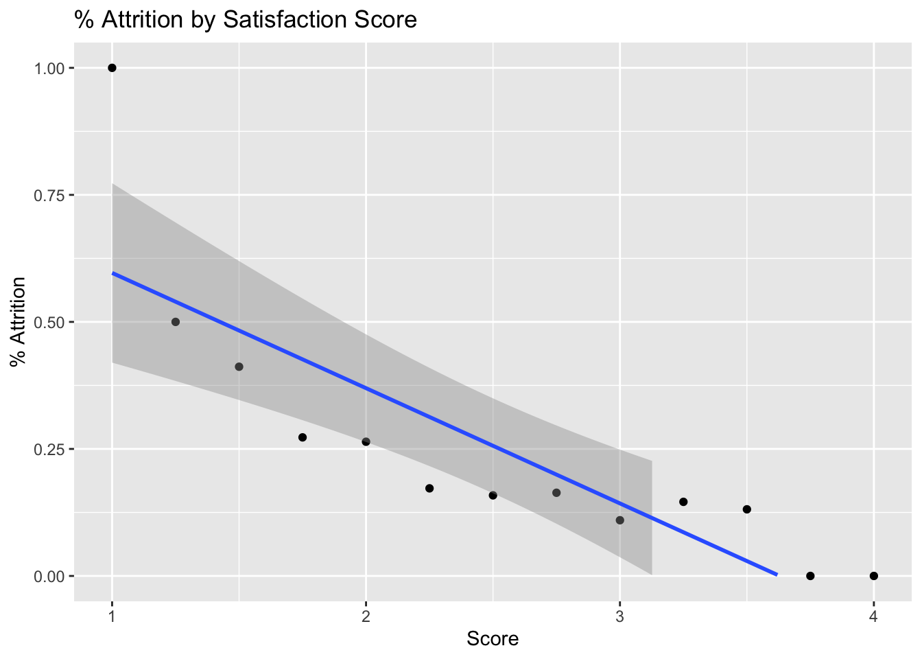

Involvement Score vs % Attrition

data = data %>%
  mutate(Involvement = (JobInvolvement+TrainingTimesLastYear+StockOptionLevel)/3)

data %>%
  group_by(Involvement) %>%
  summarize(perc_attrition = sum(Attr)/n()) %>%
  ggplot(aes(x = Involvement, y = perc_attrition)) +
  geom_point() +
  geom_smooth(method = "lm") +
  ggtitle("% Attrition by Involvement Score") +
  xlab("Score") +
  ylab("% Attrition") +
  theme(legend.position = "none")

## `geom_smooth()` using formula 'y ~ x'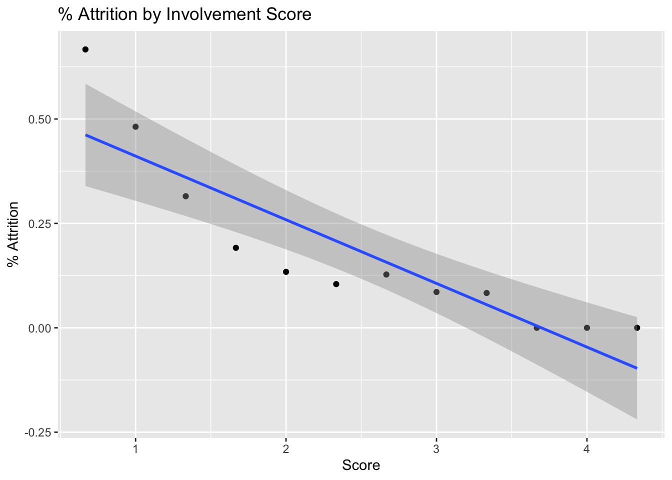

Testing Naive Bayes and Linear Regression Model

Import and Transform Data

class = read.csv("/Users/elyjiahpotter/Desktop/CaseStudy2CompSet No Attrition.csv")
linear = read.csv("/Users/elyjiahpotter/Desktop/CaseStudy2CompSet No Salary.csv")

# Adjust to include an Attr column (dummy column to maintain dataset architecture)
class = class %>%
  mutate(Attr = 0)

age_factor = cut(class$Age, breaks = c(13,19,29,39,49,59,69,79,89), labels = c("Teens", "Twenties", "Thirties", "Forties", "Fifties","Sixties","Seventies","Eighties"))

class = class %>%
  mutate(age_range = age_factor)

class = class %>% 
  mutate(age_order = case_when(
    grepl("Teens",age_range) ~ 1,
    grepl("Twenties",age_range) ~ 2,
    grepl("Thirties",age_range) ~ 3,
    grepl( "Forties",age_range) ~ 4,
    grepl("Fifties",age_range) ~ 5,
    grepl("Sixties",age_range) ~ 6
  ))

class = class %>%
  mutate(OverallSatisfaction = (JobSatisfaction+EnvironmentSatisfaction+WorkLifeBalance+RelationshipSatisfaction)/4) %>%
  mutate(Involvement = (JobInvolvement+TrainingTimesLastYear+StockOptionLevel)/3)

class2 = select_if(class,is.numeric)
class2 = class2[,1:31]

class2_not = select(class,!is.numeric)

class2_not = class2_not %>% 
  mutate(BusinessTravelRank = case_when(
    grepl("Non-Travel", BusinessTravel) ~ 0,
    grepl("Travel_Rarely", BusinessTravel) ~ 1,
    grepl("Travel_Frequently", BusinessTravel) ~ 3
  )) %>%
  mutate(DepartmentRank = case_when(
    grepl("Research & Development", Department) ~ 1,
    grepl("Human Resources", Department) ~ 2,
    grepl("Sales", Department) ~ 3
  )) %>%
  mutate(EducationFieldRank = case_when(
    grepl("Life Sciences", EducationField) ~ 1,
    grepl("Medical", EducationField) ~ 2,
    grepl("Marketing", EducationField) ~ 3,
    grepl("Technical Degree", EducationField) ~ 4,
    grepl("Other", EducationField) ~ 5,
    grepl("Human Resources", EducationField) ~ 6
  )) %>%
  mutate(GenderRank = case_when(
    grepl("Male", Gender) ~ 0,
    grepl("Female", Gender) ~ 1
  )) %>%
  mutate(OvertimeRank = case_when(
    grepl("Yes", OverTime) ~ 0,
    grepl("No", OverTime) ~ 1
  ))

class2_not = select_if(class2_not,is.numeric)
  
class2 = cbind(class2,class2_not)

gg_miss_var(class2)

## Warning: It is deprecated to specify `guide = FALSE` to remove a guide. Please use `guide = "none"` instead.

linear = linear %>%
   mutate(Attr = case_when( Attrition == "Yes" ~ 1,
                           Attrition == "No" ~ 0))

age_factor = cut(linear$Age, breaks = c(13,19,29,39,49,59,69,79,89), labels = c("Teens", "Twenties", "Thirties", "Forties", "Fifties","Sixties","Seventies","Eighties"))

linear = linear %>%
  mutate(age_range = age_factor)

linear = linear %>% 
  mutate(age_order = case_when(
    grepl("Teens",age_range) ~ 1,
    grepl("Twenties",age_range) ~ 2,
    grepl("Thirties",age_range) ~ 3,
    grepl( "Forties",age_range) ~ 4,
    grepl("Fifties",age_range) ~ 5,
    grepl("Sixties",age_range) ~ 6
  ))

linear = linear %>%
  mutate(OverallSatisfaction = (JobSatisfaction+EnvironmentSatisfaction+WorkLifeBalance+RelationshipSatisfaction)/4) %>%
  mutate(Involvement = (JobInvolvement+TrainingTimesLastYear+StockOptionLevel)/3)

linear2 = select_if(linear,is.numeric)
linear2 = linear2[,1:30]

linear2_not = select(linear,!is.numeric)

linear2_not = linear2_not %>% 
  mutate(BusinessTravelRank = case_when(
    grepl("Non-Travel", BusinessTravel) ~ 0,
    grepl("Travel_Rarely", BusinessTravel) ~ 1,
    grepl("Travel_Frequently", BusinessTravel) ~ 3
  )) %>%
  mutate(DepartmentRank = case_when(
    grepl("Research & Development", Department) ~ 1,
    grepl("Human Resources", Department) ~ 2,
    grepl("Sales", Department) ~ 3
  )) %>%
  mutate(EducationFieldRank = case_when(
    grepl("Life Sciences", EducationField) ~ 1,
    grepl("Medical", EducationField) ~ 2,
    grepl("Marketing", EducationField) ~ 3,
    grepl("Technical Degree", EducationField) ~ 4,
    grepl("Other", EducationField) ~ 5,
    grepl("Human Resources", EducationField) ~ 6
  )) %>%
  mutate(GenderRank = case_when(
    grepl("Male", Gender) ~ 0,
    grepl("Female", Gender) ~ 1
  )) %>%
  mutate(OvertimeRank = case_when(
    grepl("Yes", OverTime) ~ 0,
    grepl("No", OverTime) ~ 1
  ))

linear2_not = select_if(linear2_not,is.numeric)
  
linear2 = cbind(linear2,linear2_not)

gg_miss_var(linear2)

## Warning: It is deprecated to specify `guide = FALSE` to remove a guide. Please use `guide = "none"` instead.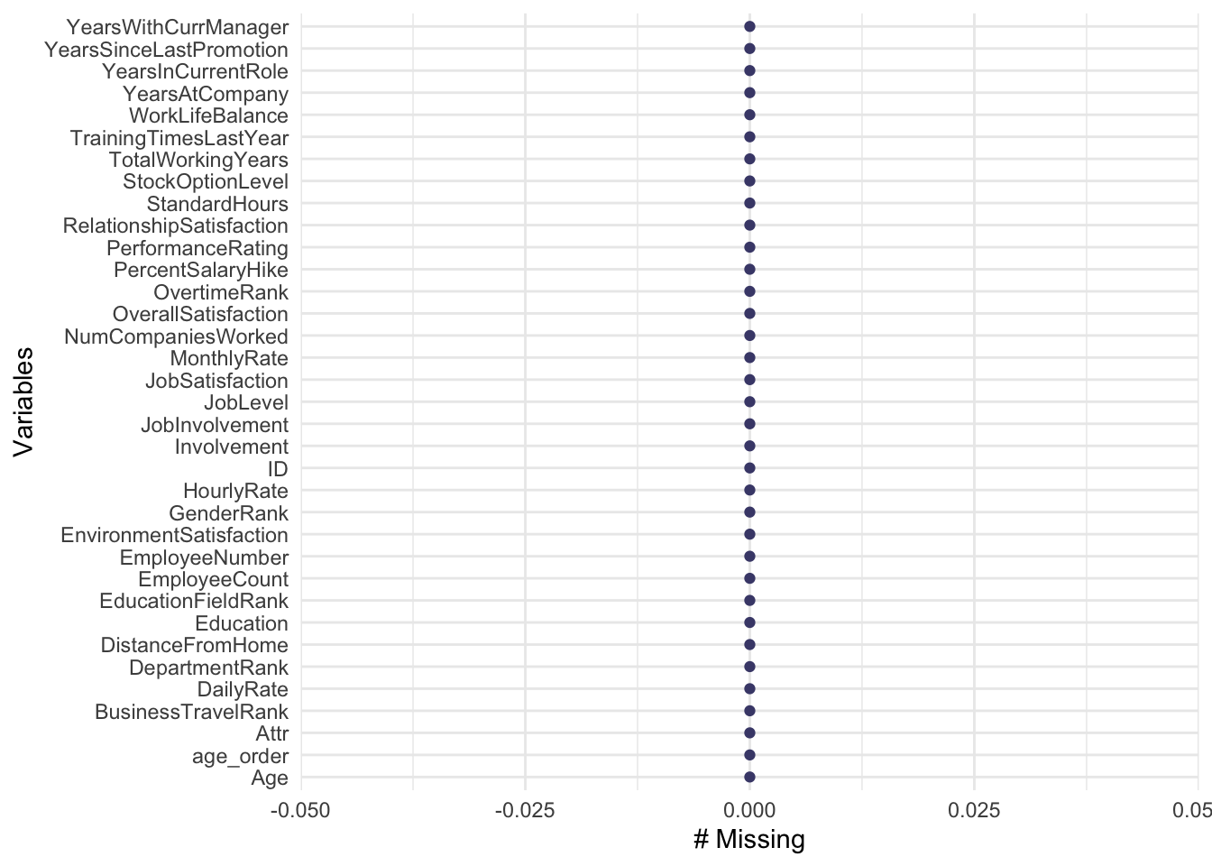

Test Classification Model

predict(bayes_model, class2)

##   [1] 0 0 1 0 0 0 0 0 0 0 1 0 0 0 0 0 0 0 0 0 0 0 0 1 0 0 1 1 1 1 1 0 0 1 1 0 0 0 0 0 0 0 0 0 1 0 0 0 0 0 0 0 0 0 0 0 0 0 0 0 0 0 1 0 0 1
##  [67] 0 0 0 0 0 0 0 0 0 1 0 0 0 0 0 0 0 0 0 0 0 0 0 1 0 0 0 0 0 0 0 0 0 1 0 0 0 0 1 0 0 0 1 0 1 0 0 0 0 0 0 0 0 0 0 0 0 0 0 0 0 0 0 0 0 0
## [133] 0 1 0 0 0 0 0 1 0 0 0 0 0 0 1 1 0 0 0 0 0 0 1 0 1 1 0 0 0 1 0 0 0 0 0 1 0 0 1 0 1 0 0 0 0 0 0 0 1 0 0 0 0 0 0 1 0 0 0 0 0 0 0 1 1 0
## [199] 0 0 0 0 0 0 0 1 0 0 0 0 1 0 0 0 0 0 0 0 0 0 0 0 0 0 1 0 0 0 1 0 1 1 0 1 0 0 0 0 0 0 0 0 0 0 0 1 1 0 0 0 1 0 0 0 0 0 0 0 1 0 0 0 0 0
## [265] 0 0 0 0 1 0 1 1 0 1 1 0 1 0 1 0 1 0 0 0 1 1 1 1 1 1 0 0 1 0 1 0 0 1 0 0
## Levels: 0 1

results = data.frame(table(class2$ID,predict(bayes_model,class2)))

colnames(results) = c("ID", "No Attrition", "Attrition")

head(results)

##     ID No Attrition Attrition
## 1 1171            0         1
## 2 1172            0         1
## 3 1173            0         0
## 4 1174            0         1
## 5 1175            0         1
## 6 1176            0         1

write.csv(results, "/Users/elyjiahpotter/Desktop/CaseStudy2_Classification_Results.csv")

Test Linear Regression Model

testing_data = linear2 %>%
  select(JobLevel, age_order, DepartmentRank)

results = data.frame(linear2$ID,predict(lin_fit, newdata = testing_data))

colnames(results) = c("ID", "Predicted Monthly Salary")

head(results)

##    ID Predicted Monthly Salary
## 1 871                 6054.134
## 2 872                 2381.020
## 3 873                14162.485
## 4 874                 2381.020
## 5 875                 2215.125
## 6 876                 5888.239

write.csv(results, "/Users/elyjiahpotter/Desktop/CaseStudy2_LinearRegression_Results.csv")

DDS-Project-2

Elyjiah Potter

11/24/2021

Case Study 2 EDA

Import Data

Check for missing values

Adjust Attrition Variable for Modeling

Investigate Distributions of Potentially Relevant Discrete Variablees

Investigate Distributions of Potentially Relevant Categorical Variables

Age Breakdown

Satisfaction Score Creation

Involvement Score Creation

Percent Attrition by key Discrete attributes

Percent Attrition by key Categorical attributes

Education Field Attrition

Education Field Satisfaction

Position Attrition

Position Avg Satisfaction

Gender / Age Attrition

Gender / Age Avg Satisfaction

Gender / Age / Marital Status Attrition

Investigating Relationship betweeen Income, Satisfaction, and Job Level

Investigate Key Categorization Attributes

Use constant value Over18 for y value for consistent comparison

Clean up data for modeling

Classification: KNN

Classification: Naive Bayes

Linear Regression Model Investigation for correlation

Top Attributes:

Collinearity

Linear Regression Model with Top 3 correlating attributes

Testing other regression combinations

Findings: JobLevel, age_order and DepartmentRank yield the lowest RMSE from the attribute set combinataions that are not collinear

Final Linear Regression Model

Top Three Factors for Attrition

Age vs % Attrition

Satisfaction Score vs % Attrition

Involvement Score vs % Attrition

Testing Naive Bayes and Linear Regression Model

Import and Transform Data

Test Classification Model

Test Linear Regression Model